
Genetic Algorithm (GA)
Modeled after the evolutionary process theory.
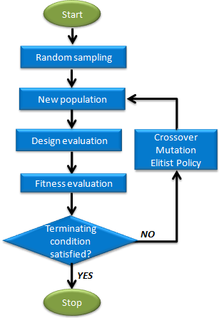
Genetic Algorithm starts with the creation of a population of designs (a generation). These designs are then ranked with respect to their fitness. Fitness is a measure of how good a design is and it is calculated as a function of constraint violation and objective function values. Selected designs are then reproduced through the application of genetic operators, typically crossover and mutation. The individuals that result from this process (the children) become members of the next generation. This process is repeated for many generations until the evolution of a population converges to the optimal solution.
Usability Characteristics
- Genetic Algorithm differs from conventional optimization
techniques in the following ways:
- They are classified as exploratory methods.
- They work on a population of designs at once.
- The design population can be run in parallel.
- They do not show the typical convergence of other optimization algorithms. You will typically select the maximum number of iterations (generations) to be evaluated. A number of solver runs is executed in each generation, with each run representing a member of the population.
- Genetic Algorithm does a global search.
- They are well suited for discrete problems.
- Genetic Algorithm is computationally expensive as it requires a large number of runs. In HyperStudy, a local search algorithm (Hooke-Jeeves or a response surface method) is utilized to improve the efficiency of Genetic Algorithm.
- In HyperStudy, population size is calculated automatically according to the optimization problem that you defined. It can also be modified manually.
- In HyperStudy, both a binary and a real coded Genetic Algorithm exists. Default is the real coded Genetic Algorithm as it is more efficient than the binary coded Genetic Algorithm.
- Genetic Algorithm terminates if one of the conditions below are
met:
- The change of the objective function during several successive iterations (as controlled by the Global search setting) is less than 0.1%.
- The maximum number of allowable iterations (Maximum Iterations) is reached.
- An analysis fails and the Terminate optimization option is the default (On Failed Evaluation).
- Supports input variable constraints.
- Although the number of evaluations per iteration is a combination of multiple settings, it is primarily affected by the Population Size setting. All evaluations within an iteration may be executed in parallel. To take advantage of parallel computation and muli-execution, set the hybrid algorithm to the meta model based method.
Settings
| Parameter | Default | Range | Description |
|---|---|---|---|
| Maximum Iterations | 200 | >0 | Maximum number of iterations allowed. |
| Minimum Iterations | 25 |
|
Processes at least Minimum Iterations iteration steps. Use this setting to prevent pre-mature convergence. By setting Minimum Iterations to be the same as Maximum Iterations, the defined number of iteration steps will be run. |
| Population Size | 0 | Integer > 1 |
If Population Size is 0, then
population size is calculated according to the following equation, where
N is the number of input variables.
If the allowable
computational effort is limited, set your own value.
Tip: In
general, it is better to process at least 25 iteration
steps. |
| Global Search | 2 |
|
Controls the global search ability. Requires ast least 0.1% improvement in the objective of the most recent M iterations or terminates when M is 5 times this setting. |
| On Failed Evaluation | Terminate optimization |
|
|
| Parameter | Default | Range | Description |
|---|---|---|---|
| Type | Real | Real or Binary |
|
| Discrete States | 1024 | Integer > 1 |
Number of discrete values
uniformly covering the range of continuous variables including upper and
lower bound.
Tip: Select as a power of 2, for example 64 =
2^6, 1024 =2^10, and so on. A larger value allows for higher
solution precision, but more computational effort is needed to find the
optima. |
| Mutation Rate | 0.01 | 0.0-1.0 |
Mutation rate (probability).
Larger values introduce a more random effect. As a result, the algorithm
can explore more globally but the convergence could be slower.
Tip: Recommended range: 0.001 – 0.05 |
| Elite Population (%) | 10 | 1.0-50.0 |
Percentage of population
that belongs to elite. The one with highest fitness value is directly
passed to the next generation. This is a very important strategy, as it
ensures the quality of solutions be non-decreasing. A larger value means
that more individuals will be directly passed to the next generation,
therefore new gene has less chance to be introduced. The convergence
speed could be increased. The drawback is that too large of values could
cause premature convergence.
Tip: Recommended range: 1.0 –
20.0. |
| Random Seed | 1 | Integer 0 to 10000 |
Controlling repeatability of
runs depending on the way the sequence of random numbers is
generated.
|
| Number of Contenders | 2 | Integer 2 to 5 |
Number of contenders in a tournament selection. For larger values, individuals with lower fitness value have less chance to be selected. Thus, the good individuals have more chance to produce offspring. The bad effect is that, diversity of the population is reduced. The algorithm could converge prematurely. |
| Penalty Multiplier | 2.0 | >0.0 |
Initial penalty multiplier
in the formulation of the fitness function as exterior penalty function.
Penalty multiplier will be increased gradually with iterating steps
going on. In general, larger values allow the solution to become
feasible with less iteration steps; but too large of a value could
result in a worse solution.
Tip: Recommended range: 1.0 –
5.0. |
| Penalty Power | 1 |
|
Penalty power in the
formulation of the fitness function as exterior penalty function.
Tip: Recommended range: 1.0 – 2.0. |
| Distribution Index | 5 | Integer 1 to 100 |
Distribution index used by real coded Genetic Algorithm. Controls offspring
individuals to be close to or far away from the parent individuals.
Increasing the value will result in offspring individuals being closer
to the parents. Tip: Recommended range: 3.0 –
10.0. |
| Max Failed Evaluations | 20,000 | >=0 | When On Failed Evaluations is set to Ignore failed evaluations (1), the optimizer will tolerate failures until this threshold for Max Failed Evaluations. This option is intended to allow the optimizer to stop after an excessive amount of failures. |
| Hybrid Algorithm | Hooke-Jeeves method |
|
Hybrid algorithm used in Genetic Algorithm. Note: This parameter is used in Genetic Algorithm real type. It is not available for binary
type. |
| Use Inclusion Matrix | With Initial |
|
|