In this tutorial, you will use SnRD to identify, evaluate,
and eliminate squeak and rattle issues.
During the first squeak and rattle screening risk analysis, input data was lacking
for the different interfaces. At that time, no gap or material properties were
defined yet. Now, the design team has more information for each of the E-Lines that
have been analyzed:
Rattle lines:
The gap and tolerances are now defined from the styling and
engineering departments.
These dimensions can now be imported into SnRD and used for updating
the existing model.
Squeak lines:
Material choices are more mature, therefore the stick slip testing
data can be searched for and applied for relevant E-Lines.
The stick slip data available in different sources (Ziegler data
base, own data base, and so on) can be imported into SnRD for
updating an existing model.
The objectives of this tutorial are:
Create FE model prepared for analyzing.
Create E-Lines using automatic and manual
methods: six rattle lines and two squeak lines.
Create a dynamic loadcase, with user defined multi direction loading
data.
Run analysis, post process, and perform sensitivity study.
Before you begin, copy the file(s) used in this tutorial to your working
directory:
In this step, you will use the Import tool to import the required
files.
From the HyperMesh NVHmenu bar, select Squeak and Rattle.
The SnRPre and SnRPost ribbons open.
From the SnRPre ribbon, select the
Import tool.
Figure 1.
Click to open additional
options.
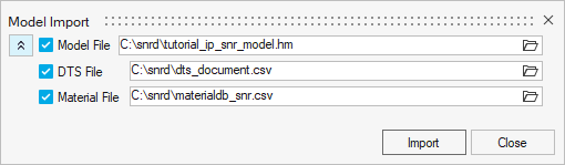
Figure 2.
Using the file browser option, browse and select files for respective
entries.
Click Import.
The selected model, DTS, and material file are imported to the
session.Figure 3.
Import Geometric Lines File
In this step, you will import the geometric lines file.
From SnRPre ribbon, select the Import
Geometry tool from the Define Interface tool group.
Figure 4.
A file browser dialog opens.
Browse and select the GeometricLines.stp file.
The geometry lines file is imported into the session.Figure 5.
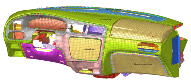
Create E-Lines
In this step, you will use the Create E-Lines tool to create
E-Lines at the interfaces.
Below are the E-Lines you will create
in this step.
Table 1.
Method
Line Type
Gap Direction
Main Component
Secondary Component
Interface Name
Manual
Rattle
Normal to Main
IP Substrate
Glove Box
GloveBox_To_IPsubstrate
Manual
Squeak
In plane to Main
IP Substrate
Dashboard Panel
Ipsubstrate_To_Dashboardpanel
Manual
Rattle
In plane to Main
Control Panel Upper
IP substrate
IPsubstrate_To_ControlpanelUpper
Manual
Rattle
Normal to Main
Radio Panel
Lower Control Panel
Radiopanel_To_ControlPanelLower
Manual
Rattle
In plane to Main
Driver Side Panel
Lower Control Panel
DriverSidepanel_To_Controlpanellower
Manual
Rattle
In plane to Main
Driver Side Panel
IP Substrate
DriverSidepanel_To_IPsubstrate
Manual
Squeak
Normal to Main
Speedometer
Control Panel Upper
Speedometer_To_ControlPanelUpper
Create E-Lines manually.
From the SnRPre ribbon, select the
Create E-Line tool.
Figure 6.
A guide bar opens.
From the guide bar, select
Manual.
By selecting the manual method, more options to create E-Lines in a more controlled manner become available on
the guide bar, see Figure 7. You must select the Main and Secondary components based on the
interface, and in which direction the local z-axis will be oriented.
However, you can select only one geometric line at a time, based on the
interface of interest.Figure 7.
For Main, select IP Substrate.
For Secondary, select Glove Box.
Tip: Press Tab to toggle between
selections.
For Line, select the geometric line present at the edge of the Glove
Box component.
Click .
E-Lines are created at the interface and will
be highlighted in yellow.Figure 8.
Repeat the substeps above to create a squeak line between the IP
Substrate and Dashboard Panel.
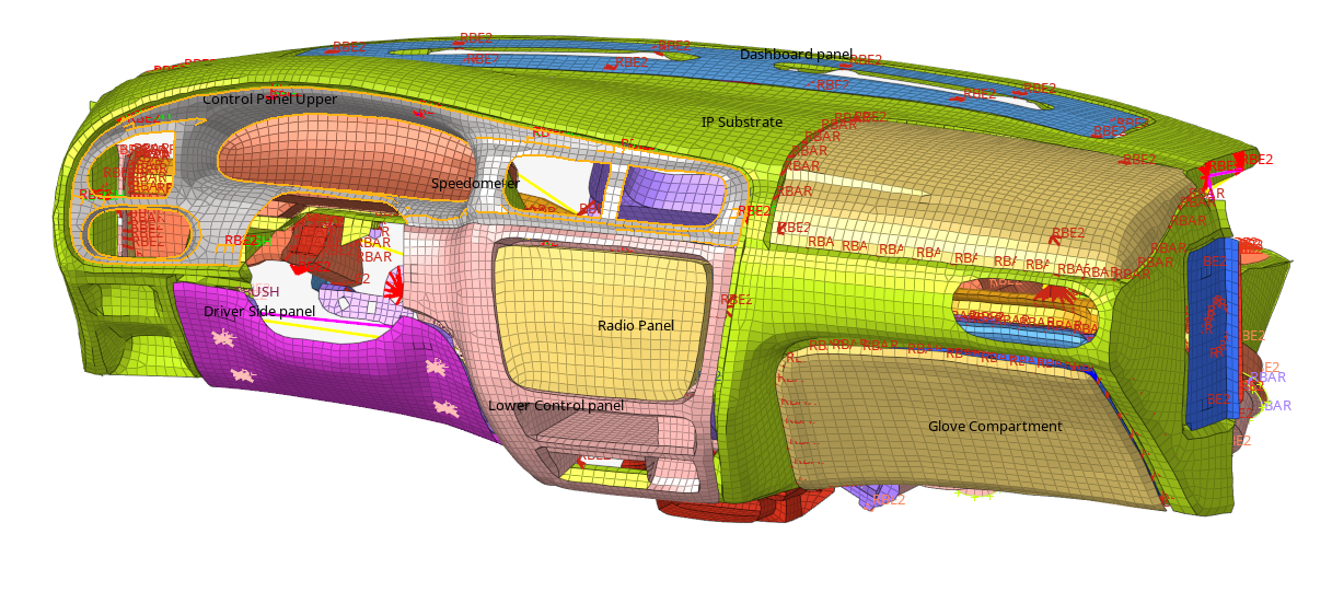
Once all E-Lines are created, your model
should look like Figure 9.Figure 9.
Realize E-Lines
In this step, you will use the Manage E-Lines tool to realize all
E-Lines.
From the SnRPre ribbon, select the Review
E-Lines tool from the Manage E-Line tool group.
Figure 10.
The Review E-Line dialog opens.
Map the correct interface from the DTS file to the created E-Lines and ensure all other options, like Gap direction, are
correct.
Figure 11.
Note: The E-Line status is represented using three colors:
Red indicates a failed E-Line.
Yellow indicates an unrealized E-Line.
Green indicates a fully realized E-Line.
Optional: If an E-Line status is yellow, click to realize and update E-Lines.
From the Material Mapping tab, select the following materials for the two
squeak E-Lines.
IPSubstrate_To_Dashboardpanel
For Main Material, select PPTD_20.
For Secondary Material, select
PPTD_20.
Speedometer_To_ControlPanelUpper
For Main Material, select PPTD_20.
For Secondary Material, select ABS.
Tip: In the Review E-Line dialog, click to connect to
Ziegler Database and map materials. See Ziegler PEM Material Database for
more information.
Figure 12.
Define Dynamic Loadcase
In this step, you will create a Dynamic loadcase.
From SnRPre ribbon, select the Dynamic
Event tool.
Figure 13.
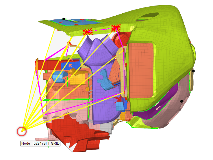
In the modeling window, select the node shown in Figure 14.
Figure 14.
A microdialog opens.Figure 15.
Verify Displacement (D) is selected as load type.
For Load Curve, select From File.
For load directions, select X, Y,
and Z.
Select Constrain all Dofs to constrain the excitation
nodes in all the other directions.
Click .
A file browser dialog opens.
Browse and select the Excitation_XYZ.csv file from the
003_loads folder.
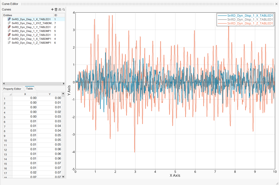
The required load collectors and other entities required for the
simulation are created. The newly created loads are displayed in the
Curve Editor dialog.
In the Curve Editor dialog, review the load curves and
close the dialog.
Figure 16. Figure 17.
Tip: You can use the Model Browser to view
the new entities.
Review Loadcase and Export Solver Deck
Review the Dynamic Loadcase.
From the SnRPre ribbon, Analyze
group, select the Review Loadcases tool.
Figure 18.
The Load Step Table dialog opens.Figure 19.
Verify the Export checkbox is enabled for the
SnRD_Dyn_Disp_#_XYZ entry.
Close the dialog.
From the SnRPre ribbon, Analyze
group, select the Export tool.
Figure 20.
The Model Export dialog opens.Figure 21.
Click Export.
A folder selection dialog opens.
Browse and select the required folder.
The OptiStruct solver deck is exported to
the selected folder.
Click Close to close the Model
Export dialog.
Use the exported .FEM solver deck to
solve in the OptiStruct solver. Once completed, two output
files are generated: .H3D and .PCH. These
files will be used in the Post Processing of results.
Post Process Results
In this step, you will perform a Full Analysis to understand the squeak and rattle risks in the model.
From the SnRPost ribbon, select the Risk
Assessment tool.
Figure 22.
The SnR Risk Assessment Browser opens.
For Result File, select the .pch file.
Note: Prior to selecting the .pch file, the
.fem and .csv file must
already be loaded in the SnRPre ribbon.
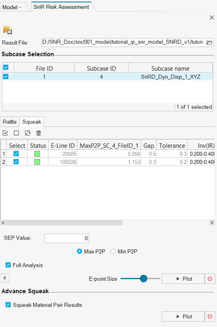
Under Subcase Selection, select the subcase.
The rattle and squeak lines are segregated into separate
tabs.
Select the line Ids required to perform post-processing.
For SEP, enter 0.
Verify Full Analysis is selected to see the line-level
plots and to continue to next steps of post-processing.
Important: You must perform full analysis to access Sensitivity
Analysis and combined loading capabilities.
Note:If
Full Analysis is not selected, only a summary
analysis is generated. Full Analysis is selected
by default.
Click Plot.
Seven pages are created
containing the details and summary for rattle analysis. You must switch to the squeak
tab and select the lines for squeak results.
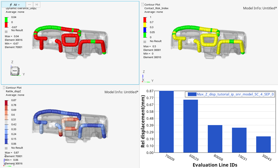
Full analysis creates 11 pages containing all the details. The summary for rattle
analysis can be found on page one.Figure 23. Rattle Summary Dynamic
To access squeak results, you must click on the squeak tab and
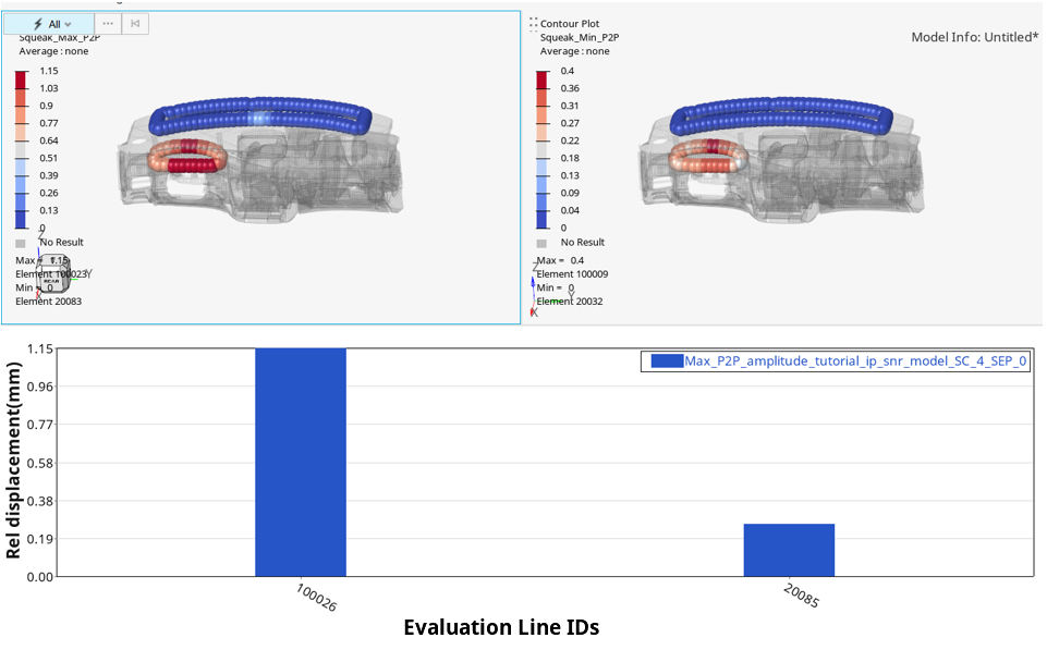
click Plot. The plots in sequence are as shown below:
Maximum Peak-to-peak Displacement plot:
Minimum Peak-to-peak Displacement plot:
Maximum P-P Displacement bar plot.
To visualize P-P displacement in comparison with the Impulse rate data from testing,
you should access advanced squeak capabilities.Figure 24. Figure 25. Squeak Summary Dynamic
Evaluate Results
In this step, you will study the histograms and contour plots to understand results
and complete squeak and rattle risk evaluation.
From page one of the Rattle Summary Dynamic, you can see the
Rattle line ID 19513009 has the maximum relative displacement. You will perform
Sensitivity Analysis to evaluate the effects of modes on the relative
displacements.
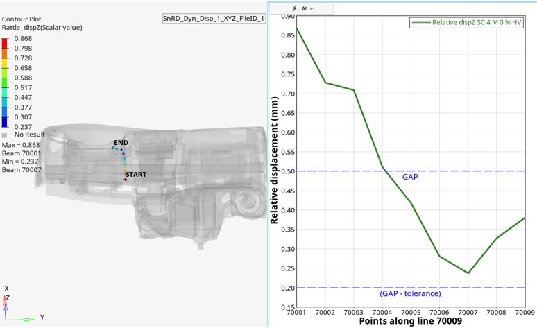
Navigate to page six to view the Rattle Detailed Dynamic - Line ID 70009
details.
Figure 26.
The Relative Displacement of 0.86 mm at the point 70001. This is higher than
the Gap and (Gap - Tolerance) values. This indicates a risk of rattle at this
particular interface of Driver Side Panel - Lower Control Panel.
From the SnRPost ribbon, select the
Sensitivity Analsysis tool.
Figure 27.
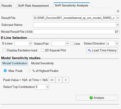
The SnR Sensitivity Analysis Browser opens.Figure 28.
Define the following parameters.
For Result File, select
Tutorial_IP_SNR_Model.pch.
For Subcase Name, select Subcase 4
(SnRD_MTRAN_EnforcedDisplacement_1_XYZ).
For Modal Result File (.H3D), select
Tutorial_IP_SNR_Model.h3d.
In the E-Line Selection section, define the following parameters.
For E-Lines, select
70009.
For Select Pair, select Line check box.
For Select Direction, select Z.
Click Load Time History.
A working window opens stating the process of plotting relative
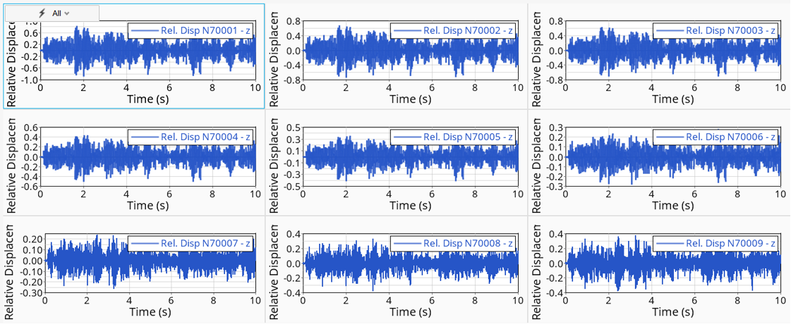
displacement.Figure 29. Once complete, the relative displacement plots for all the points in the
line are plotted.Figure 30.
Under the Modal Contribution panel, click Analyze.
A working dialog opens stating the process of plotting Relative Modal
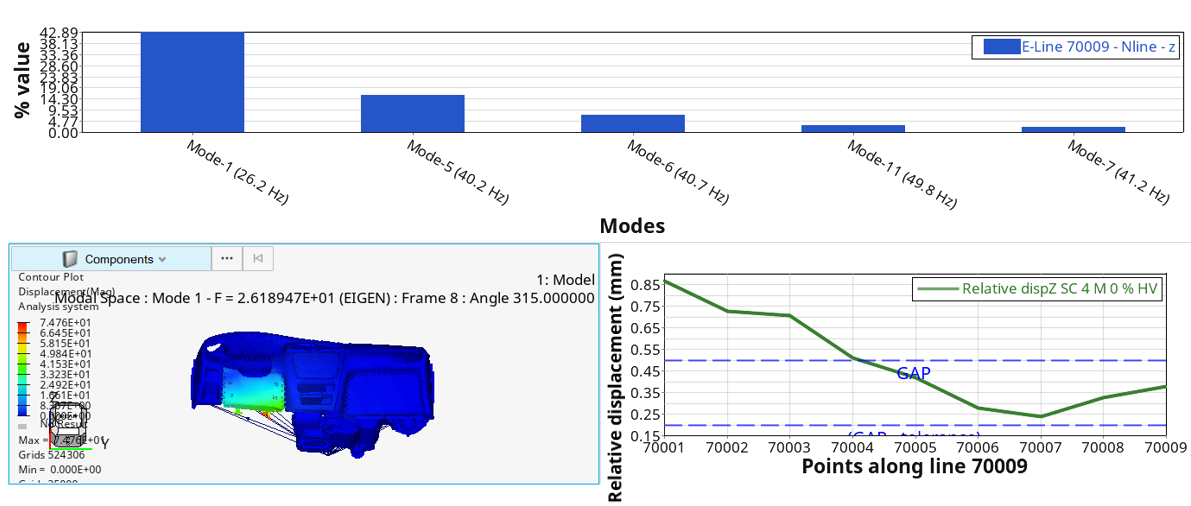
Contribution.Figure 31. Relative Modal Contribution - Line 70009 - z is created with modes,
contour and relative displacement plots for the line.Figure 32. Figure 33. From the Modes plot, the Mode-4 of value 26.5 Hz is the highest
contributing factor for the rattle issue.
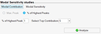
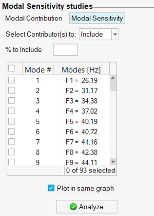
Click Modal Sensitivity under the Modal Sensitivity
Studies panel.
Figure 34.
Select Exclude from the Select Contributor(s) to
list.
Enter 50 for % to Exclude value.
Enable the checkbox for mode 4 under the Mode # column.
Click Analyze.
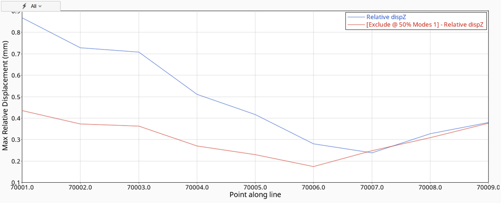
The Modal Sensitivity for Line (MSL) - Line ID 19513009 -z page is
created in the session with the Max Relative Displacement (mm) values plotted
against all the interface points.Figure 35. The relative displacement is reduced when the mode 4 is excluded by
50%.
Repeat the above steps to study the remaining lines in the model.

 to open additional
options.
to open additional
options.
 A file browser dialog opens.
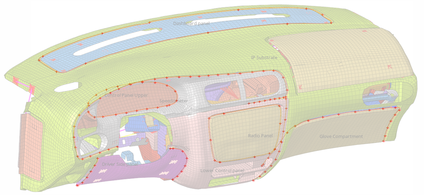
 A guide bar opens.
 .
E-Lines are created at the interface and will be highlighted in yellow.
.
E-Lines are created at the interface and will be highlighted in yellow.
 The Review E-Line dialog opens.
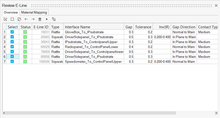
 to connect to
Ziegler Database and map materials. See Ziegler PEM Material Database for
more information.
to connect to
Ziegler Database and map materials. See Ziegler PEM Material Database for
more information.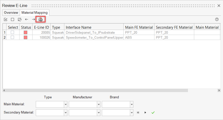

 A microdialog opens.
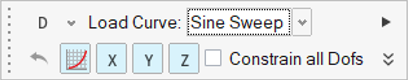
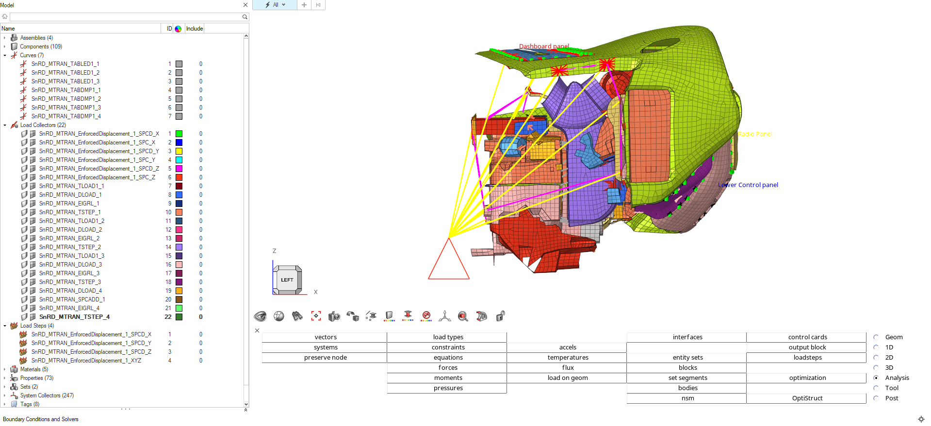 Tip: You can use the Model Browser to view the new entities.
 The Load Step Table dialog opens.
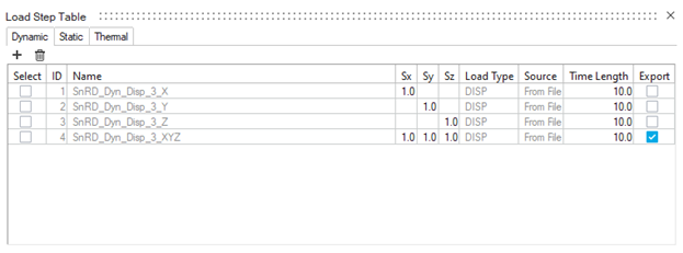
 The Model Export dialog opens.
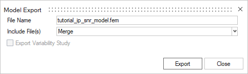

 The Relative Displacement of 0.86 mm at the point 70001. This is higher than the Gap and (Gap - Tolerance) values. This indicates a risk of rattle at this particular interface of Driver Side Panel - Lower Control Panel.