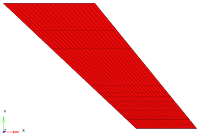
The structural domain consists of a stick model with CQUAD4
elements with linear orthotropic material properties.
E1
3.151E+09
E2
4.162E+08
NU12
0.31
G12
4.392E+08
RHO
381.980
Flutter analysis is performed for set of Mach numbers (M) = {0.35, 0.5, 0.7,
0.9} for a velocity range of [120, 330] m/s. In Figure 15 on page 65, the variation
of mass ratios across Mach number suggests difference in flow conditions across the
experiments1. Hence, the density ratios were varied for each Mach
number in separate simulations.
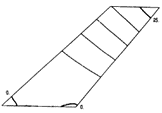
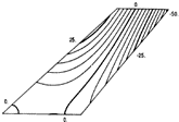
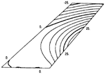
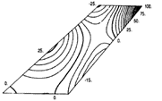
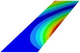
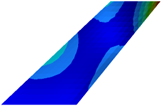
Comparison of Normal Modes
Mode shape and mode frequency comparisons are as follows. The results from OptiStruct are in agreement with the reference results1.
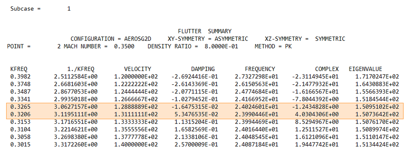
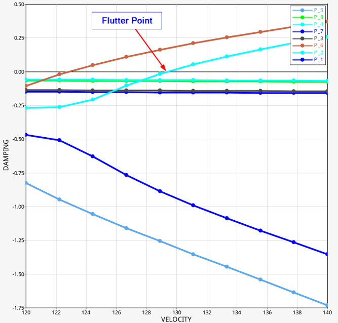
From the .flt file of the first Mach number (M = 0.35)
simulation, the flutter point (where damping changes sign) corresponding to the
lowest mode is identified as the 2nd mode with a velocity between 128.89
m/s to 131.12 m/s.
Note: By definition, instability (flutter or divergence) occurs
when the damping values are zero. At this point, if the frequency is zero, then
the instability is due to divergence. Otherwise, the instability is due to
flutter.
Figure 2. Flutter Analysis Summary from .flt
File Plotting the v-g curve, the velocity at this flutter point is 129.417 m/s.
This is the most critical flutter point that needs to be avoided for M = 0.35.Figure 3. Identify Flutter Points. The flutter point corresponding to the lowest velocity is also visually
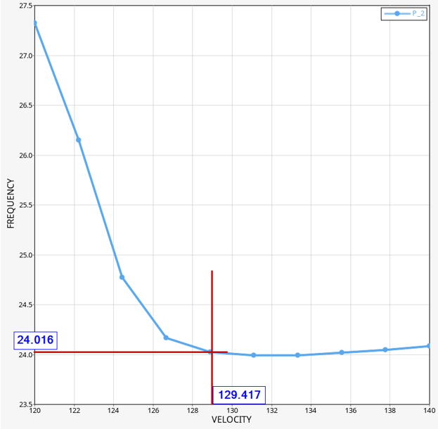
identified. Figure 4. Identify Frequency Value at Critical Flutter Point from v-f
Curve Plotting the v-f plot for the 1st mode (corresponding to the critical flutter
point), the frequency value for 1st mode at a velocity of 129.417 m/s is
determined as 24.016 Hz. In the same way, the flutter speed and flutter frequency
determination was repeated for M = {0.5, 0.7, 0.9}.
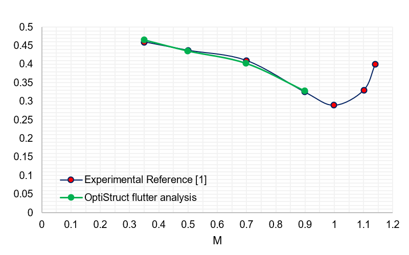
Comparison of Flutter Speed Coefficient
The flutter speed coefficient is calculated from OptiStruct and plotted against M and compared against the
reference plot from Figure 16(a) on page 661.
Where,
Flutter velocity
Streamwise semi chord length at wing root = m
Natural circular frequency of the first uncoupled torsional mode rad/s (This is the 2nd normal
mode for this wing)
Mass ratio
This value was determined for each Mach number from Figure 15 on page
651
Figure 5. Flutter Speed Coefficient versus M Comparison Between
Experimental Reference and OptiStruct Flutter
Analysis
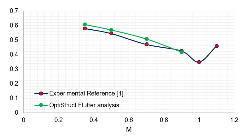
Comparison of Flutter Frequency Ratio
The flutter frequency ratio is calculated from OptiStruct and plotted against M. This is compared against
the reference plot from Figure 16(b) on page 671.
Figure 6. Flutter Frequency Ratio versus M Comparison Between
Experimental Reference and OptiStruct Flutter
Analysis
Observations
The flutter speed coefficient and flutter frequency ratio from OptiStruct are in close agreement with the
experimental reference data.
The current support of OptiStruct Aeroelastic
Analysis is limited to Subsonic flow (M < 1.0) and hence the simulations
were not performed beyond M = 0.9. The support for supersonic regime is
planned for a future release and Figure 5 and Figure 6 will be updated with the pertinent data points in this
regime.
In realistic conditions, for M ~ 0.75 and above, local pockets of supersonic
flow could occur around the structure. This intermediate regime is denoted
as transonic.
In the flutter speed coefficient versus M plot, the experimental reference
data shows a reduction in flutter speed coefficient around M = 1.0 and this
is called the transonic dip.
OptiStruct flutter analysis is capable of
capturing the descent of this dip.
Figure 7. Transonic Dip
Reference
1
E. Carson Yates Jr, “AGARD Standard Aeroelastic Configurations for Dynamic
Response. Candidate Configuration I.-WING 445.6,” NASA Technical Memorandum
I00492. 1987