OS-HM-T: 5010 Linear Transient Heat Transfer Analysis of an Extended Surface Heat
Transfer Fin
This tutorial outlines the procedure to perform a linear transient heat transfer
analysis on a steel extended-surface heat transfer fin attached to the outer surface of a
system generating heat flux (for example, an IC Engine).
Before you begin, copy the file(s) used in this tutorial to your
working directory.
The extended surface heat transfer fin analyzed in this tutorial is one of many from
an array of such fins connected to the system. The fins draw heat away from the
outer surface of the system and dissipate it to the surrounding air. The process of
heat transfer out of the fin depends upon the flow of air around the fin (free or
forced convection). In the current tutorial, the focus is on transient heat transfer
through heat flux loading and free convection dissipation. An extended surface heat
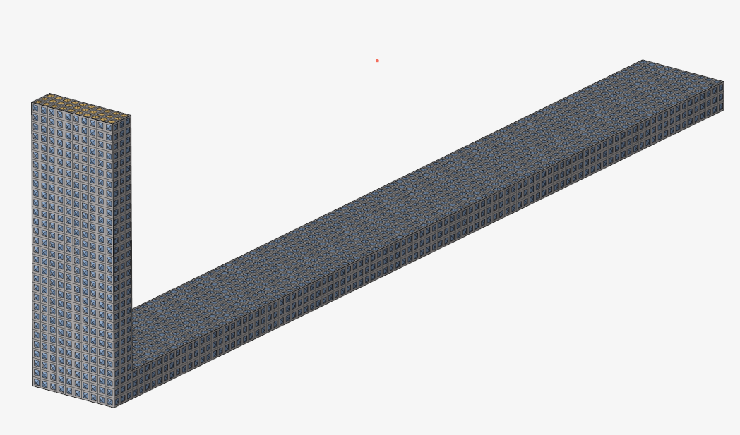
transfer fin made of steel is illustrated in Figure 1. To meet certain structural design requirements, the fin is bent
at 90° at approximately a quarter of its length.
Note: A free convection analysis is
conducted in this tutorial. However, if forced fluid flow (forced convection) is
allowed over the outer surface of the system, offsetting the fins from each
other periodically interrupts the growth of a thermal boundary layer and a
reduction in flow velocity occurs due to form drag, resulting in a higher heat
transfer rate.
Figure 1. Extended Surface Heat Transfer Fin for Convective and Conductive
Transient Heat Transfer
The extended surface heat transfer fin is meshed with CHEXA
elements in HyperMesh and a transient heat transfer
analysis is performed in HyperMesh using the OptiStruct solver. A typical heat flux load of 100
KW/m2 is applied to the face connected to the outer surface of the
system. An ambient temperature of 25°C is assumed and all material properties are
assumed to remain constant with temperature and time. Free (Natural) convection is
assumed over the entire surface of the material, wherein heat transfer between the
surface of the fin and the surrounding air occurs due to a complex mechanism of
density differences resulting from temperature gradients.
Checkpoint:
Steady-state heat transfer analysis is generally sufficient for a wide variety of
applications. However, in situations where the system properties vary significantly
over time and this variation needs to be captured for the intended application, the
transient nature of heat transfer must be considered. Some examples are the
relatively slow heating of airplane gas turbine compressor disks compared to the
turbine casing leading to aerodynamic issues during takeoff, or the analysis of the
time taken for the onset of frostbite in fingers or toes.
The following exercises are included:
Create the thermal material and the solid property for the given
component
Assign the material and property to the component
Create flux and convective loads and boundary conditions for the model
Submit the job to OptiStruct
Post-process the results using HyperView
Launch HyperMesh
Launch HyperMesh.
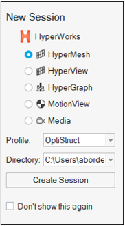
In the New Session window, select HyperMesh from the list of tools.
For Profile, select OptiStruct.
Click Create Session.
Figure 2. Create New Session This loads the user profile, including the appropriate template, menus,
and functionalities of HyperMesh relevant for
generating models for OptiStruct.
Import the Model
On the menu bar, select File > Import > Solver Deck.
In the Import File window, navigate to and select
heat_transfer_fin.fem you saved to your
working directory.
Click Open.
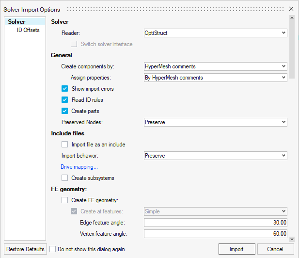
In the Solver Import Options dialog, ensure the Reader is
set to OptiStruct.
Figure 3. Import Base Model in HyperMesh
Accept the default settings and click Import.
Set Up the Model
Create Thermal Material and Properties
The imported model only contains the component and predefined element sets for
boundary condition creation. Create a thermal material that can be assigned to this
component.
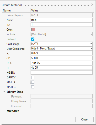
In the Model Browser, right-click and select Create > Material.
A default MAT1 material displays in a
Create Material window.
For Name, enter steel.
Select the check box next to MAT4.
In the Create Material window, enter the following values
for the material, steel:
[K] Thermal conductivity = 7.3 x 10⁻² W/mm °C
[CP] Heat capacity at constant pressure = 508 J/Kg °C
[RHO] Material density = 7.9 x 10⁻⁶ Kg/mm3
[H] Heat transfer coefficient = 4 x 10⁻⁵ W/mm2 °C
Figure 4.
Click Close.
This is purely a heat transfer analysis, so structural properties (for
example, the MAT1 card) are not required. It is assumed that
the thermal material properties (MAT4) are temperature
independent.
A new material, steel, is created with thermal properties necessary for
a transient heat transfer analysis. Next, create the solid property for this
model referencing the PSOLID entry and connect the material,
steel, to this property; the property can then be assigned to the existing
component.
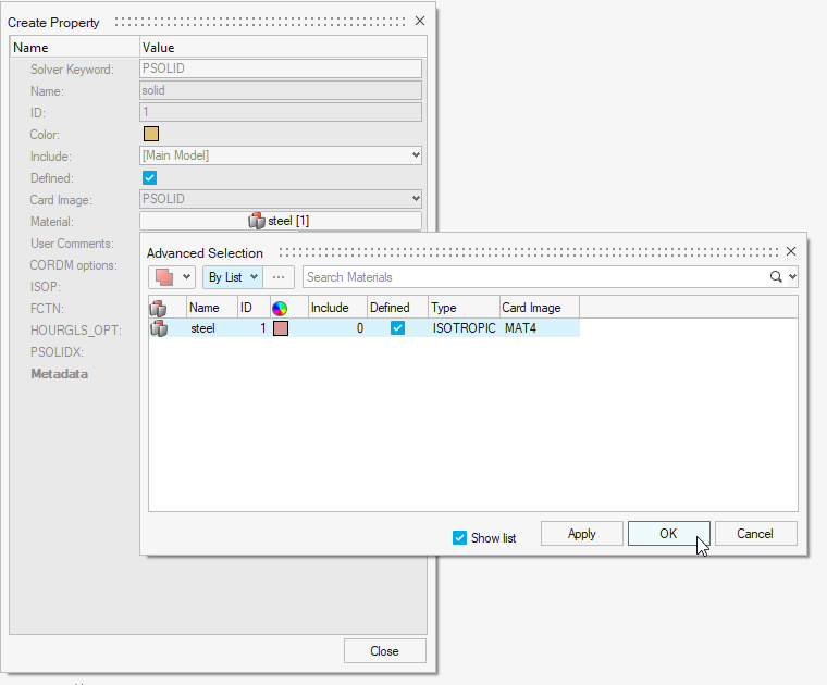
In the Model Browser, right-click and select Create > Property.
A default PSHELL property displays in a
Create Property window.
For Name, enter solid.
For Card Image, select PSOLID from the drop-down
menu.
For Material, click Unspecified.
Click .
In the Advanced Selection window, select
steel and click OK.
Click Close.
The property of the steel fin is created as 3D
PSOLID. Material information is linked to this property.Figure 5.
Link the Material and Property to the Existing Structure
Once the material and property are defined, they need to be linked to the
structure.
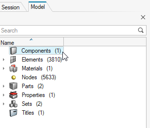
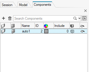
In the Model Browser, double click
Components to open the Components browser.
Figure 6. Select auto1 Component
Click on the auto1 component.
The component template displays in the Entity Editor.
For Property, click Unspecified.
Click .
In the Advanced Selection window, select
solid and click OK.
Figure 7. Select solid Property
Create Time-steps for the Transient Heat Transfer Analysis
A transient analysis captures the behavior of the system over a specific period of
time. Therefore, a time period of interest for your system is defined. A time period
of 500 seconds (8 minutes, 20 seconds) is defined with results output every 10
seconds. A load collector is created for this purpose and the
TSTEP entry is referenced.
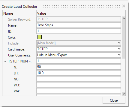
In the Model Browser, right-click and select Create > Load Collector.
For Name, enter Time Steps.
For Card Image, select TSTEP.
For TSTEP_NUM, enter a value of 1.
For the number of time steps (N), enter 50
Set each time increment (DT) to 10.
This encompasses a total time period of 500 seconds in which to capture
the behavior of the system.Figure 8. TSTEP Entry Options
Click Close.
Create Initial Conditions for the Transient Heat Transfer Analysis
Since the temperature profile of the system varies over time, the initial grid point
temperature profile must be set to specify the starting point for the analysis.
Assume that the temperature of the entire system is equal to 25°C at T = 0 seconds;
the TEMPD Bulk Data Entry sets the initial temperatures.
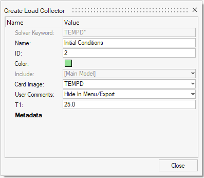
In the Model Browser, right-click and select Create > Load Collector.
For Name, enter Initial Conditions.
For Card Image, select TEMPD.
For T1, enter 25.
Click Close.
Figure 9. Initial Condition
Apply Ambient Temperature Boundary Conditions
Ambient temperature thermal boundary conditions are applied on the
model by creating specific load collectors for each. The ambient temperature is
controlled using an SPCD entry, as this allows an ambient
temperature variation over time to help mimic such physical requirements (if
any).
Create the SPCD Entry for Time-variant Ambient Temperature
A time-variable ambient temperature can be created by referencing an
SPCD entry via a TLOAD1 load step input
data entry. The time variable nature of the ambient temperature can be captured
using a TABLED1 entry also referenced by the
TLOAD1 data.
In the Model Browser, right-click and select Create > Load Collector.
For Name, enter Ambient SPCD.
For Card Image, select None.
The newly created Ambient SPCD load collector becomes the current load
collector.
Click Close.
Create the Amplitude
Create the amplitude (constant part) of the time variant ambient temperature using an
SPCD data entry.
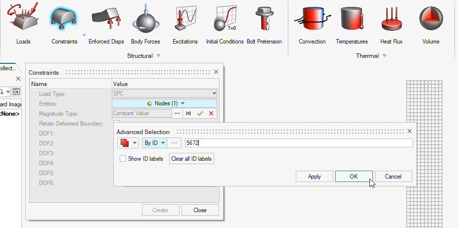
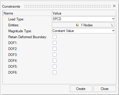
From the Analyze ribbon, select Constraints.
For Entities, select Nodes > .
In the Advanced Selection window, select By
ID from the drop-down menu.
In the text box, enter 5672 and click
OK.
Figure 10. SPCD on Ambient Node
For Load Type, select SPCD from the drop-down
menu.
Clear the check boxes for DOF1,
DOF2, DOF3,
DOF4, DOF5, and
DOF6.
Click Create and Close.
Figure 11. SPCD Input
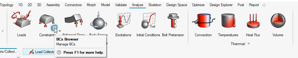
From the Constraints tool group, select the BCs Browser
satellite icon.
Figure 12. BC Browser Access
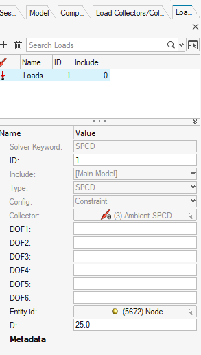
In the Loads Browser, select Loads.
For the SPCD constraint, D field, enter 25.0.
This creates an SPCD referencing the ambient node specifying a
temperature of 25°C.Figure 13. SPCD Definition
Create a Curve
Create a curve to define the time variant nature of the ambient temperature. This is
done by creating a TABLED1 entry.
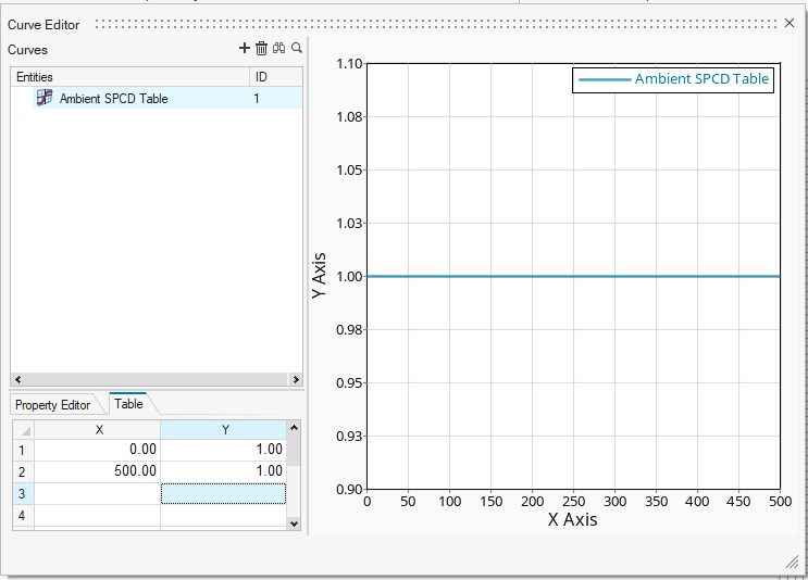
In the Model Browser, right-click and select Create > Curve.
A new Curve Editor window opens.
For Name, enter Ambient SPCD Table.
In the table, enter the following values:
x(1) = 0.0
y(1) = 1.0
x(2) = 500.0
y(2) = 1.0
Figure 14. Ambient SPCD Curve
Close the editor.
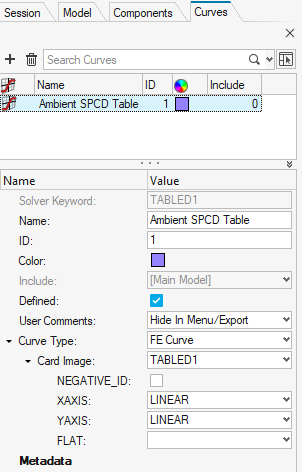
In the Model Browser, double-click on curves to open
the Curves Browser.
Select Ambient SPCD Table.
In the Entity Editor, change the card image from TABDMP1 to
TABLED1.
Note: In this tutorial, a constant ambient temperature (the values of y(1) and
y(2) are the same leading to a constant temperature distribution over the
first 500 seconds) is defined; this demonstrates the procedure to use a
TABLED1 entry to specify a time variant ambient
temperature as well. To do this, specify different values for the y# fields
and depending on the type of variation required, select from
LINEAR or LOG
options.
Figure 15. Ambient SPCD Curve
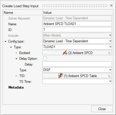
Create Load Step Inputs
In the Model Browser, right-click and select Create > Load Step Inputs.
For Name, enter Ambient SPCD TLOAD1.
For Config Type, select Dynamic Load - Time
Dependent.
For Type, select TLOAD1 from the drop-down menu.
The SPCD and its corresponding
TABLED1 table are linked to the TLOAD1
entry.Figure 16. Process to Specify Time-Variant SPCD
For EXCITEID, select the Ambient SPCD load
collector.
For TYPE, select DISP,
Click TID and select the Ambient SPCD
Table from the curve menu.
Click Close.
Figure 17. Define TLOAD Load Step Input
Create SPC Data Entries
All entities referenced by SPCD entries should also be constrained
by SPC data entries. The value of the corresponding
SPC referencing an ambient point controlled via an
SPCD by TLOAD1/TLOAD2
entries should be equal to zero (0.0).
Create a new load collector named Ambient SPC.
For Card Image, select None.
From the Analyze ribbon, select Constraints.
For Entities, select Nodes > .
In the Advanced Selection window, select By
ID from the drop-down menu.
In the text box, enter 5672 and click
OK.
Clear the check boxes for DOF1,
DOF2, DOF3,
DOF4, DOF5, and
DOF6.
Click Create and then
Close.
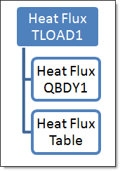
Apply a Heat Flux Load
Ambient temperature thermal boundary conditions are assigned to the model and heat
flux load from the outer surface of the engine (to which the fin is attached) is
applied next on the model. A time-varying heat flux load of 0 to 0.1
W/mm2 from 0 to 500 seconds is used for the analysis of this fin.
This load is applied on the model by creating specific load collectors for the
corresponding TLOAD1, QBDY1 and
TABLED1 entries similar to the procedure used for the ambient
temperature SPCD definition.
Create the QBDY1 Entry for Time-variant Heat Flux Load
A time variable heat flux load can be created by referencing an
QBDY1 entry via a TLOAD1 load step input
data entry. The time variable nature of the heat flux load can be captured using a
TABLED1 entry also referenced by the
TLOAD1 data.
In the Model Browser, right-click and select Create > Load Collector.
For Name, enter Heat Flux QBDY1.
For Card Image, select None.
Click Close.
Create the Heat Flux Load
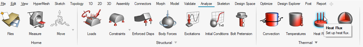
From the Analyze ribbon, click Heat Flux.
Figure 18. Select Heat Flux Load
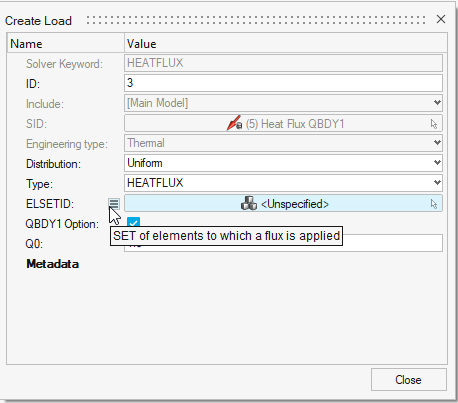
In the Create Load window, next to ELSETID, click > Create.
Figure 19. Choose Surface for Heat Flux Load You can create a SURF SET on which the heat flux is applied.
For Name, enter flux_surf.
For Elements, select 0 Elements then switch to
Faces in the drop-down menu.
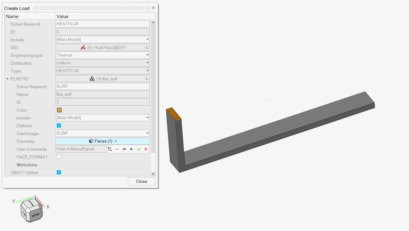
Hover over and select the faces automatically highlighted in the short end of
the fin.
With this method, you can easily select the faces on which heat flux is
applied.Figure 20. Select Surfaces for Heat Flux Load
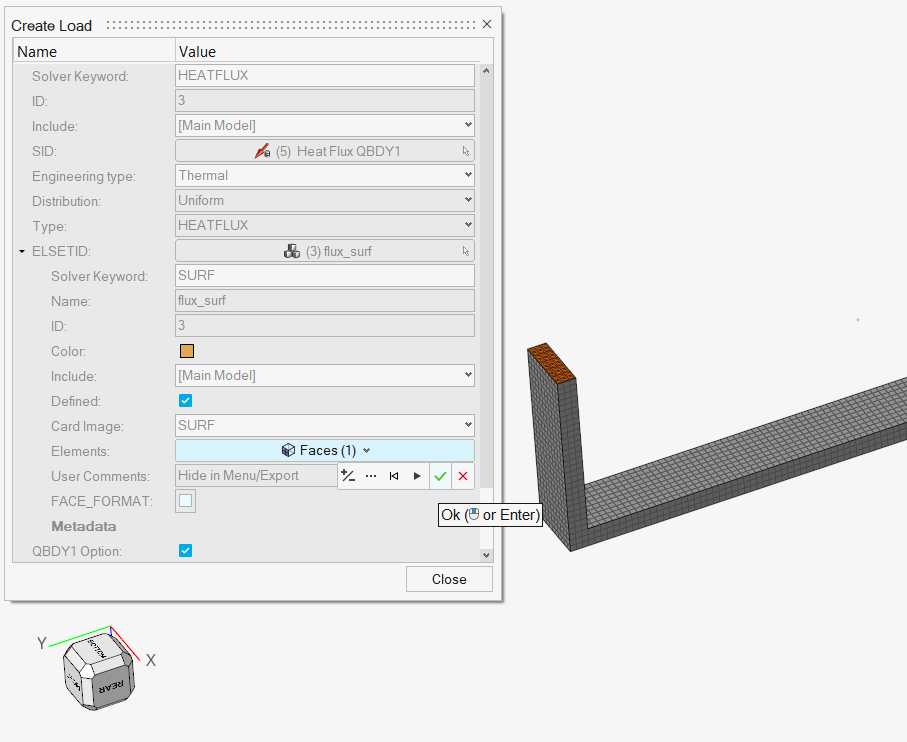
Once the faces are selected, click .
Figure 21. Finalize Selection
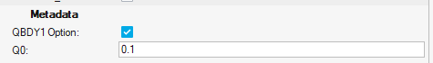
For QBDY1 Option, Q0 field, enter 0.1.
Figure 22. Apply Heat Flux Load Value
Click Close.
Create a Curve
Create a curve to define the time variant nature of the heat flux load. This is done
by creating a TABLED1 entry.
In the Model Browser, right-click and select Create > Curve.
A new Curve Editor window opens.
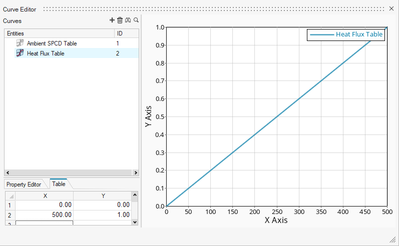
For Name, enter Heat Flux Table.
In the table, enter the following values:
x(1) = 0.0
y(1) = 0.0
x(2) = 500.0
y(2) = 1.0
Figure 23. Heat Flux Table
Close the editor.
In the Model Browser, double-click on curves to open
the Curves Browser.
Select Heat Flux Table.
In the Entity Editor, change the card image from TABDMP1 to
TABLED1.
Note: In this tutorial, a linearly incremental heat flux load is defined (the
values of y(1) and y(2) are 0 and 1 leading to a linearly increasing heat
flux distribution over the first 500 seconds).
Create Load Step Inputs
In the Model Browser, right-click and select Create > Load Step Inputs.
For Name, enter Heat Flux TLOAD1.
For Config Type, select Dynamic Load - Time
Dependent.
For Type, select TLOAD1 from the drop-down menu.
The QBDY1 and its corresponding table are linked to
the TLOAD1 entry.Figure 24. Process to Specify Time-variant Heat Flux Load
For EXCITEID, select the Heat Flux QBDY1 load
collector.
For TYPE, select LOAD,
Click TID and select the Heat Flux
Table from the curve menu.
Click Close.
Figure 25. Define Time-Varying Heat Flux Loading via TLOAD1
Add Free Convection
Free convection is assigned in a similar manner to the procedure used for the
creation of the conduction interface. Free convection is, however, automatically
assigned to all heat transfer subcases and the PCONV and
CONV entries should refer to the material, steel, and the
ambient temperature. The difference between the ambient temperature and the
structural surface temperature allows for calculation of the amount of heat
transferred through free convection.
Create Surface Elements for Free Convection
Surface elements are created to simulate the heat exchange between the fin surface
and the surrounding air.
In the Model Browser, right-click and select Create > Load Collector.
For Name, enter free convection.
For Card Image, select None.
Click Close.
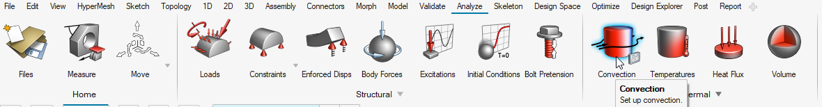
From the Analyze ribbon, clickConvection.
Figure 26. Select Convection Load
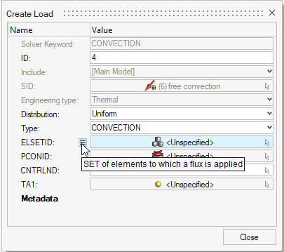
For ELSETID, select > Create.
Figure 27. Choose Surfaces for Convection Load You can create a SURF SET which contains the faces participating in free
convection heat transfer.
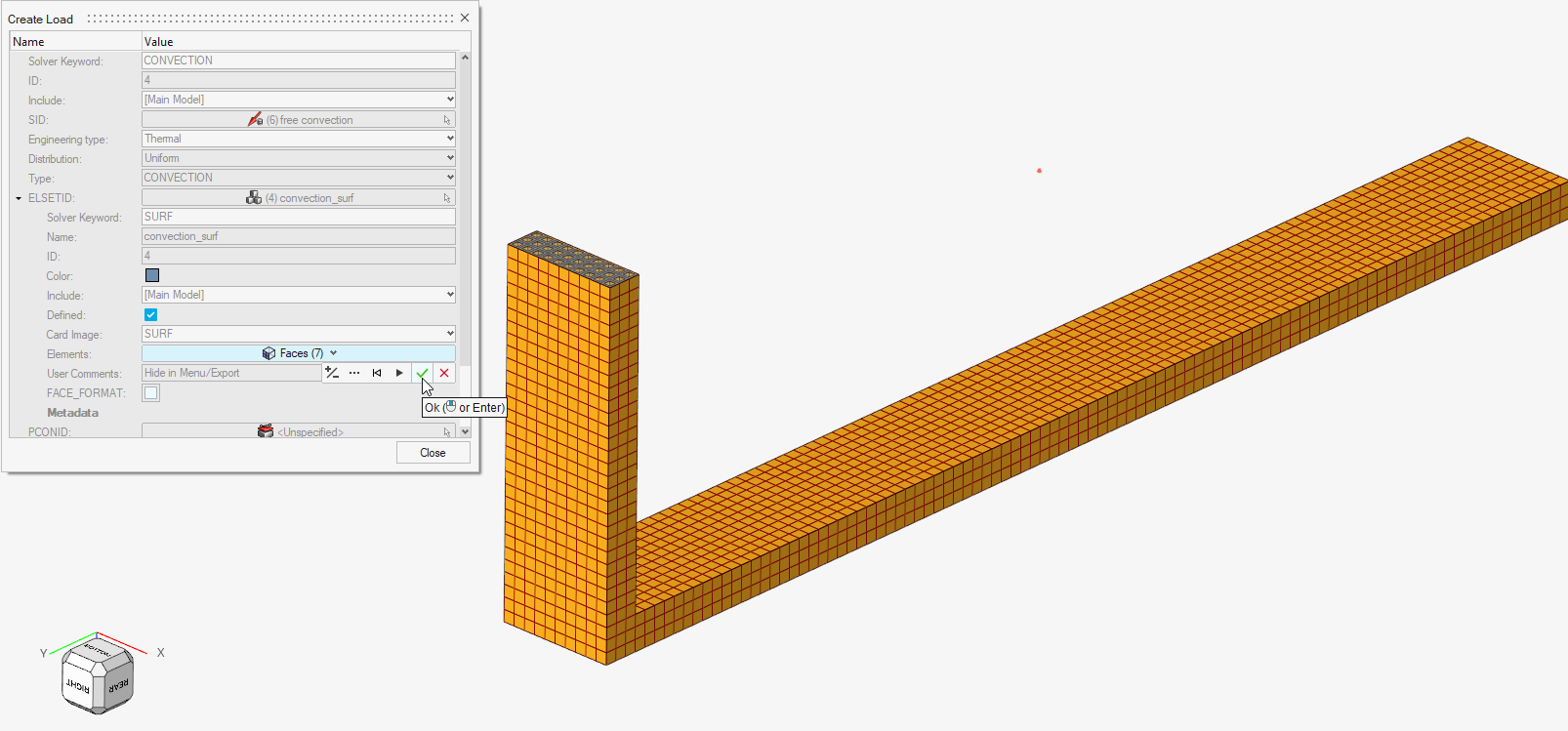
For Name, enter convection_surf.
For Elements, select 0 Elements then switch to
Faces in the drop-down menu.
Hover over and select all faces that are not part of the previously defined
heat flux input surface.
After the required faces are selected, click .
Figure 28. Finalize Surfaces for Free Convection Heat Transfer
The convection surface elements are displayed in blue and the conduction
heat flux surface elements are displayed in orange in this model as seen in the
image below (the colors are arbitrary based on the assigned color of the
SURF entries, and may differ in your model).Figure 29. Review Conduction (Heat Flux) and Convection Surface Elements
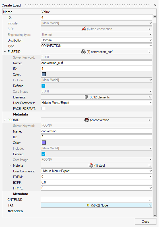
Next to PCONID, select > Create.
For Name, enter convection.
For Material, click Unspecified > to open Advanced Selection.
Select Steel and click OK.
For TA1, click Unspecified > to open Advanced Selection.
Select By ID from the drop-down menu and enter node ID
5672 in the text box.
This sets the convection boundary condition by identifying the
convection ambient point for free convection ambient temperature definition.
Figure 30. Final Free-Convection Definition
Click Close.
Combine TLOAD Entries Into One DLOAD Entry
Two different TLOAD1 entries are defined and since they are to be referenced in the
same subcase, they should be combined using a DLOAD Bulk Data
Entry.
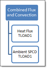
In the Model Browser, right-click and select Create > Load Step Inputs.
For Name, enter Combined Flux and Convection.
For Config Type, select Dynamic Load Combination.
The default Type is DLOAD.
For S, enter 1.0.
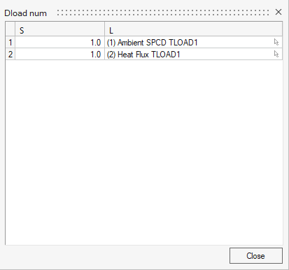
As only a simple linear addition of the two TLOAD1 entries
is required, for DLOAD_NUM, enter 2 and press
Enter.
Click .
In the pop-up window, enter S(1) = 1.0 and S(2) =
1.0.
For L(1), select Ambient SPCD TLOAD1.
For L(2), select Heat Flux TLOAD1.
The DLOAD entry is created as a linear combination of
two TLOAD1 entries – Heat Flux TLOAD1 and
Ambient SPCD TLOAD1. Figure 31. Process to Specify Time-variant SPCD Figure 32. Combination of Two TLOAD Entries on One DLOAD
Click Close twice.
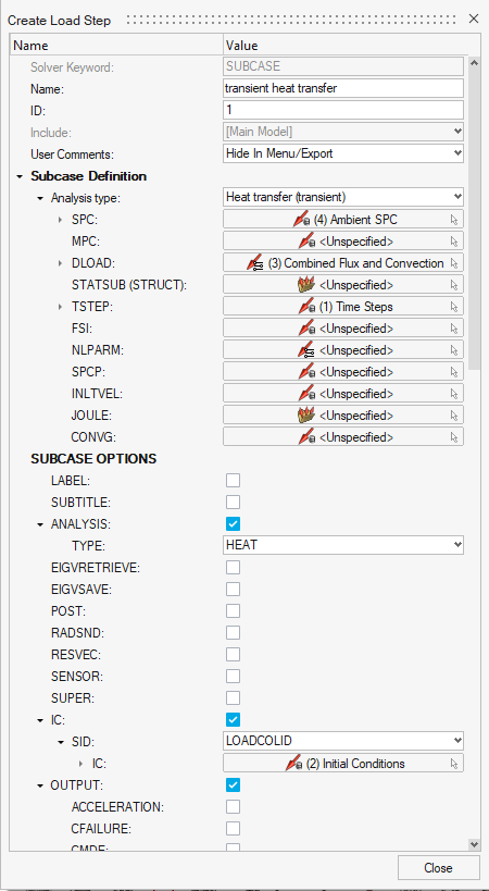
Create a Transient Heat Transfer Load Step
An OptiStruct transient heat transfer load step is
created which references the time steps in the Time Steps load collector, the
initial conditions in the Initial Conditions load collector, the heat flux and free
convection setup in the Combined Flux and Convection load collector, and the SPC
boundary condition in the Ambient SPC load collector. The gradient, flux, and
temperature output for the heat transfer analysis are also requested.
In the Model Browser, right-click and select Create > Load Step Inputs.
For Name, enter transient heat transfer.
For Analysis type, select Heat transfer (transient) from
the drop-down menu.
For SPC, select Unspecified > Loadcol.
In the Advanced Selection dialog, select
Ambient SPC as the SPC and click
OK.
For TSTEP, select Time Steps.
For DLOAD, select Combined Flux and Convection.
In the SUBCASE OPTIONS, select the IC check box.
Select LOADCOLID from the drop-down menu..
Click on Unspecified and select Initial
Conditions.
Select the Output check box.
On the sub-list, select the THERMAL and
FLUX options.
For both options, set the FORMAT field to H3D.
For both options, set the OPTION field to ALL.
Figure 33. Linear Transient Heat Transfer Subcase Information
Click Close.
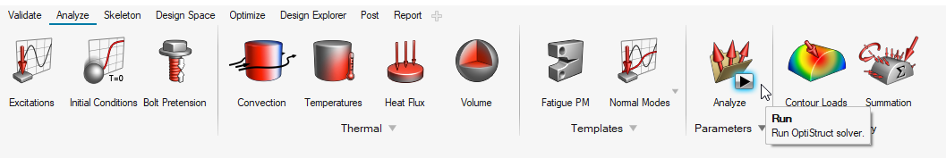
Run OptiStruct
On the Analyze ribbon, under the Analyze tool group, select Run OptiStruct Solver.
Figure 34. Initiate the OptiStruct Analysis Run
In the File Explorer, save the model as heat_transfer_fin_complete to your working directory.
The .fem filename extension is the recommended extension
for OptiStruct input decks.
Click Save.
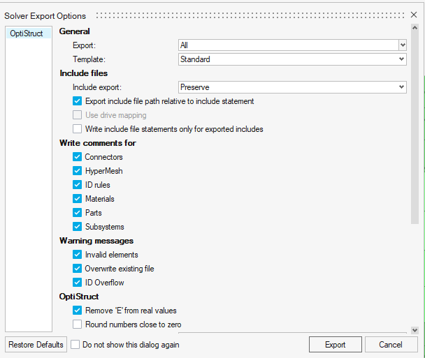
In the Solver Export Options window, for Export, select
All and accept all other default settings.
Click Export.
Figure 35. Export Completed OptiStruct Input File
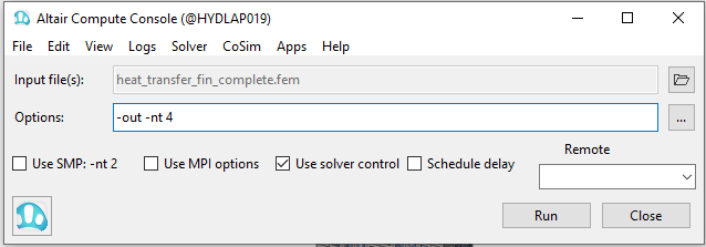
In the Altair Compute Console, for Options, add the
following run options:
Figure 36. Altair Compute Console
Click Run.
Once the job completes successfully, the ACC Solver View
window opens and an ANALYSIS COMPLETE message is printed in the Message
log.
Click Close.
If the job is successful, you should see new results files in the
directory in which heat_transfer_fin_complete.fem was
run. The heat_transfer_fin_complete.out file is a good
place to look for error messages that could help debug the input deck if any
errors are present.
View Transient Heat Transfer Analysis Results
When the message Process completed successfully is received in the command
window, click Results.
HyperView is launched and the results are loaded.
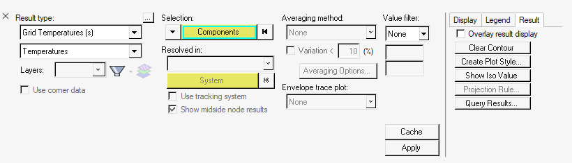
For Result type, in the first drop-down menu, select Grid
Temperatures(s).
Figure 37. Contour Plot Panel HyperView
Click Apply.
From the Results Browser, select Time = 5.0000000E+02.
A contour plot of grid temperatures at the final time step is
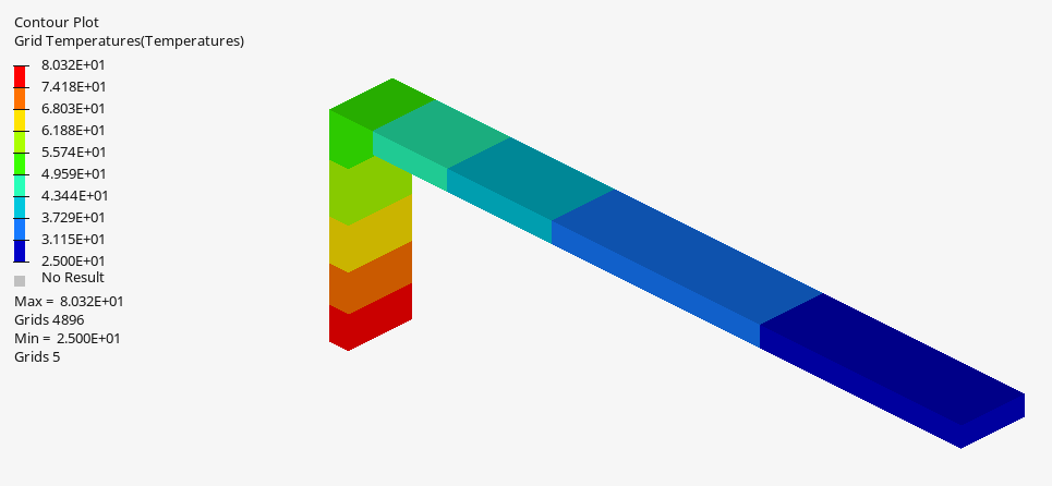
created.Figure 38. Grid Temperature Contour for Final Time Step (500 seconds) WITH FREE
CONVECTION
This is the grid point temperature plot after 500 seconds. The system
is input a linearly increasing heat flux from 0 to 0.1 W/mm2 from
0 to 500 seconds respectively. Therefore, a physical correlation can be the
effect of starting an IC engine to full capacity wherein the flux
transmitted to the outer surface linearly increases with time.
Note: The flux
patterns in actuality may be different and may fluctuate based on the
duration of the power cycles. The maximum temperature of 80.32°C
predictably occurs at the elements closest to the heat flux loading site
and the minimum temperature of 25.0°C occurs at elements farthest from
the heat source.
From the Results Browser, select Time = 4.6000000E+02.
A contour plot of grid temperatures is created.Figure 39. Grid Temperature Contour after 460 Seconds WITH FREE
CONVECTION
For Results type, first drop-down menu, select Element Fluxes
(V).
Click Apply.
From the Results Browser, select Time = 5.0000000E+02 to
view the element flux results after 500 seconds.
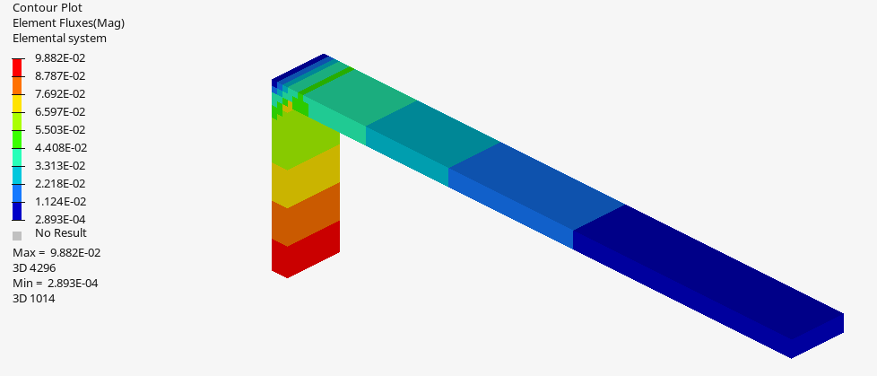
Figure 40. Element Flux Results after 500 seconds WITH FREE CONVECTION
In a practical setting, you can also see the effect of free convection in the
reduction of temperature at the outer surface of the system. Convection (due
to the extended surface area) allows a larger amount of heat to be drawn out
of the system when compared to the absence of an extended surface fin. This
is evident in the temperature of the outer surface of the system after 500
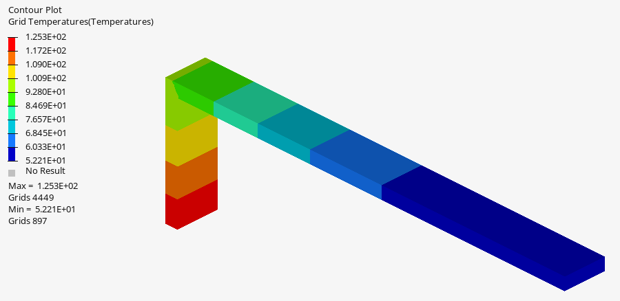
seconds in the absence of convection heat loss.Figure 41. Grid Temperature Contour after 500 seconds WITHOUT FREE
CONVECTION
The maximum temperature at the outer surface of the heat source system is
125.3°C, which decreases by around 45°C to 80.3°C when free-convection is
included. Therefore, using an extended surface fin is a very effective way
to reduce the temperature of a system.

 .
.

 Constraints.

 Heat Flux.
 > Create.
 .
.

 Convection.
 .
.
 Run OptiStruct Solver.