Sequential Quadratic Programming (SQP)

A gradient-based iterative optimization method and is considered to be the best method for nonlinear problems by some theoreticians. In HyperStudy, Sequential Quadratic Programming has been further developed to suit engineering problems.

Usability Characteristics

A gradient-based method, therefore it will most likely find the local optima.
One iteration of Sequential Quadratic Programming will require a number of simulations. The number of simulations required is a function of the number of input variables since finite difference method is used for gradient evaluation. As a result, it may be an expensive method for applications with a large number of input variables.
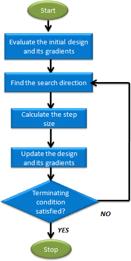
Sequential Quadratic Programming terminates if one of the conditions below are met:
- One of the two convergence criteria is satisfied.
  - Termination Criteria is based on the Karush-Kuhn-Tucker Conditions.
  - Input variable convergence
- The maximum number of allowable iterations (Maximum Iterations) is reached.
- An analysis fails and the Terminate optimization option is the default (On Failed Evaluation).
The number of evaluations in each iteration is automatically set and varies due to the finite difference calculations used in the sensitivity calculation. The number of evaluations in each iteration is dependent of the number of variables and the Sensitivity setting. The evaluations required for the finite difference are executed in parallel. The evaluations required for the line search are executed sequentially.

Figure 1. Sequential Quadratic Programming Process Phases

Settings

In the Specifications step, change method settings from the Settings and More tabs.

Note: For most applications the default settings work optimally, and you may only need to change the Maximum Iterations and On Failed Evaluation.

Table 1. Settings Tab
Parameter	Default	Range	Description
Maximum Iterations	25	> 0	Maximum number of iterations allowed.
Design Variable Convergence	0.0	>=0.0	Input variable convergence parameter. Design has converged when there are two consecutive designs for which the change in each input variable is less than both (1) Design Variable Convergence times the difference between its bounds, and (2) Design Variable Convergence times the absolute value of its initial value (simply Design Variable Convergence if its initial value is zero). There also must not be any constraint whose allowable violation is exceeded in the last design. Note: A larger value allows for faster convergence, but worse results could be achieved. $\begin{array}{l} {\begin{matrix} \| x_{j}^{i} - x_{j}^{i - 1} \| < γ \cdot (x_{j}^{U} - x_{j}^{L}) \\ {\begin{matrix} \| x_{j}^{i} - x_{j}^{i - 1} \| < γ \cdot \| x_{j}^{0} \|, {if(x}_{j}^{0} \neq 0) \\ \| x_{j}^{i} - x_{j}^{i - 1} \| < γ, {if(x}_{j}^{0} =0) \end{matrix} \\ c_{\max}^{k} \leq g_{\max} \end{matrix} \\ i = k, k - 1; j = 1, 2, ..., n \end{array}$ Where, $x$ is input variable; $x^{0}$ is the initial design; $x^{L}$ , $x^{U}$ are lower bound and upper bound of input variables respectively; $k$ is the current iteration number; $n$ is the number of input variables; $y$ is the input variable convergence parameter.
On Failed Evaluation	Terminate optimization	Terminate optimization Ignore failed evaluations	Terminate optimization Terminates with an error message when an analysis run fails. Ignore failed evaluations Ignores the failed analysis run. If analysis is failed at line search then the step size is reduced by half and the optimization is continued; if analysis is failed at gradient calculation then the corresponding gradient is set to zero (an exception is that if the gradient calculation is failed on all of the input variables, then Sequential Quadratic Programming will be terminated).

Table 2. More Tab
Parameter	Default	Range	Description
Termination Criteria	1.0e-4	>0.0	Defines the termination criterion, relates to satisfaction of Kuhn-Tucker condition of optimality. Recommended range: 1.0E-3 to 1.0E-10. In general, smaller values result in higher solution precision, but more computational effort is needed. For the nonlinear optimization problem: $\begin{array}{l} \begin{matrix} \min & f (x) \\ g_{i} (x) \leq 0 \\ s . t . & h_{j} (x) = 0 \end{matrix} \\ i = 1, ..., m; j = 1, ..., 1 \end{array}$ Sequential Quadratic Programming is converged if: $\| S^{T} \cdot \nabla f \| + \sum_{i = 1}^{m} \| μ_{i} \cdot g_{i} \| + \sum_{j = 1}^{l} \| λ_{j} \cdot h_{j} \| \leq Δ$ Where $S$ is the search direction generated by Sequential Quadratic Programming; $\nabla f$ is objective function gradient; $μ, λ$ are Lagrange multipliers; $Δ$ is the value of the termination criteria parameter.
Sensitivity	Forward FD	Forward FD Central FD Asymmetric FD Analytical	Defines the way the derivatives of output responses with respect to input variables are calculated. Forward FD For approximation by one step forward finite difference scheme. $d f / d x = (f (x + d x) - f (x)) / (d x)$ Central FD For approximation by two step central (one step forward, one step back) finite difference scheme. See Equation 1. Asymmetric FD For approximation by two step non-symmetric (one step forward, half step back) finite difference scheme. See Equation 2. Tip: For higher solution precision, 2 or 3 can be used, but more computational effort is consumed.
Max Failed Evaluations	20,000	>=0	When On Failed Evaluations is set to Ignore failed evaluations (1), the optimizer will tolerate failures until this threshold for Max Failed Evaluations. This option is intended to allow the optimizer to stop after an excessive amount of failures.
Use Perturbation size	No	No or Yes	Enables the use of Perturbation Size, otherwise an internal automatic perturbation size is set.
Perturbation Size	0.0001	> 0.0	Defines the size of the finite difference perturbation. For a variable x, with upper and lower bounds (xu and xl, respectively), the following logic is used to preserve reasonable perturbation sizes across a range of variables magnitudes: If abs( x) >= 1.0 then perturbation = Perturbation Size * abs( x) If (xu - xl) < 1.0 then perturbation = Perturbation Size * (xu – xl) Otherwise perturbation = Perturbation Size
Use Inclusion Matrix	With Initial	With Initial Without Initial	With Initial Runs the initial point. The best point of the inclusion or the initial point is used as the starting point. Without Initial Does not run the initial point. The best point of the inclusion is used as the starting point.

Figure 2.

d f / d x = (f (x + d x) - f (x - d x)) / (2 * d x)

Figure 3.

d f / d x = ((f (x) + f (x + d x)) / 3 - 4 / 3 * f (x - 0.5 d x)) / d x