Overview of Fast Fourier Transform, phenomena, windowing, Filtering Frequency
Response, functions, blocking, and Hilbert Transform.
Fast Fourier Transform
The first fundamental tool of signal processing is the Fourier Transform. The Fourier
Transform is used to map time-domain data into the frequency domain. The
frequency-domain representation of a curve (or signal) contains the same information
as the time-domain representation, but in a different form. Each representation is
useful in certain circumstances. The most basic use of the frequency-domain
representation is to view the frequency content of a signal.
The equation for a Fourier Transform is:
Notice that the result is complex-valued. Normally, the
complex-valued function is represented by a magnitude and a phase angle rather than
real and imaginary components, although they are equivalent. This is because the
magnitude and phase angle have physical meaning, whereas the real and imaginary
components do not. The lower limit of the integral is usually set to zero, since
time cannot be negative in a physical sense.
In order to perform a Fourier Transform on a computer, the signal to be transformed
must be digitized. The basic requirement for all discrete Fourier Transforms is that
the discrete input data be sampled at a constant frequency, such that all time
intervals are identical. If the input data is not evenly sampled, the discrete
Fourier transform will be incorrect.
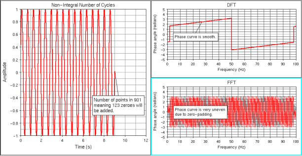
A Fast Fourier Transform (FFT) is a computationally efficient algorithm for
evaluating the Fourier Transform equation. The only additional requirement is that
the input signal have a number of points equal to two raised to some integral power:
that is, 256 (28), 512 (29), and so on. If the input signal
does not have a valid number of points, zeros are added at the end of the signal
until a valid number of points is reached. This is called
zero-padding.Figure 1. Discrete Fourier Transform and Fast Fourier Transform
HyperView, MotionView, and
HyperGraph have both a regular discrete Fourier
Transform and a Fast Fourier Transform. The advantage of the discrete Fourier
Transform is that no zero-padding occurs. This is important because zero-padding can
distort the phase angle spectrum. The advantage of the Fast Fourier Transform is in
computation speed, which varies with the number of points.
Normally, the frequency domain representation of a signal is shown in two plots: the
magnitude, or amplitude, spectrum and the phase spectrum. At any given frequency,
the magnitude and phase can be used to construct a sine wave of that frequency which
is contained in the original signal, according to the following:
If the responses at every frequency are combined, the result is
the original signal.
For example, in HyperGraph, create the following
curve:
Now
create a second curve in a different window on the same page. It should
be:
x=freq(p1w1c1.x)
y=FFTmag(p1w1c1.y)
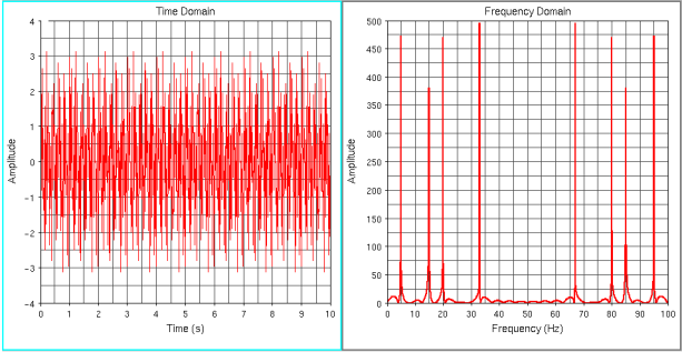
Figure 2.
The result shows spikes at each of the frequencies present in the initial equation,
that is, at 5 Hz, 15 Hz, 20 Hz, and 33 Hz.
Notice that there will also be other spikes at frequencies not present in the initial
equation, at 67 Hz, 80 Hz, 85 Hz, 95 Hz. This is due to phenomena caused by sampling
the data, and is discussed below.
Since the right half of the spectrum is essentially redundant, the left half is
normally all that is plotted. HyperGraph accounts for
this using the fold function. The right half of the spectrum is folded back onto the
left half. In the previous example, replace the y equation
with:
y = fold(FFTmag(p1w1c1.y))
Only the left half of the spectrum is shown.
FFT Phenomena
There are two separate and distinct phenomena introduced in digital signal
processing. The first is called aliasing, and is due to the sampling of
the data. The second phenomenon is known as leakage, and is due to
discontinuities at the endpoints of the signal.
Aliasing
Due to the nature of sampled data, only a limited frequency range can be
examined using discrete Fourier transforms. The valid frequency range is
from 0 to half of the sampling frequency. This is known as the Nyquist
frequency. Any frequencies outside of this range are erroneously
attributed to frequencies inside the range. These frequencies will be
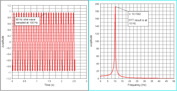
"folded" back into the valid range.Figure 3.
For example, a curve has a frequency content at 90 Hz and is sampled at
100 Hz. The Nyquist frequency is then 50 Hz. Since 90 Hz is greater than
50 Hz, it will be folded about the Nyquist frequency back into the valid
range of 0-50 Hz. Therefore, it will be mapped to 10 Hz, as well as 90
Hz (and 110 Hz, 190 Hz, ...). The spectrum is always symmetric about the
Nyquist frequency, as seen in the above example.
Leakage
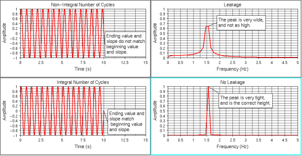
An assumption made by the Fourier Transform is that the signal being
transformed is periodic, allowing the integral in Equation 1 to go from
0 to the signal duration rather than from 0 to infinity. This means
that, in effect, the FT algorithm is concatenating the signal with
itself indefinitely. At the endpoints of the signal, discontinuities
often occur. These discontinuities are very difficult to map to periodic
components. In fact, they require an infinite number of periodic
components. This, in turn, introduces spurious frequency components into
the resultant spectrum.Figure 4. The most common method used to reduce leakage is to use data
windowing.
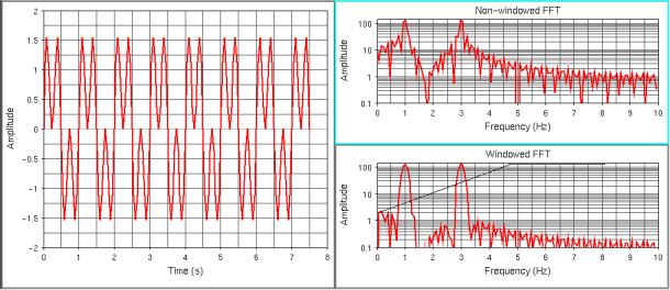
Windowing
As described in the previous section, discontinuities at the end points of the signal
introduce leakage. Leakage is undesirable because it distorts the true spectral
characteristics of the signal. To eliminate leakage, not only must the end points of
the signal have the same value, but they must also have the same slope.
The most common way to reduce leakage is by using windowing functions. A sample
windowing function is shown below. The sample shows the Hamming window function.Figure 5.
The value of the windowing function starts out very small, increases to a value of
one in the middle, and then decreases symmetrically. When this function is
multiplied by the input signal, it has the effect of damping out the ends of the
signal. Thus, when the signal is concatenated with itself, no large discontinuities
will be present since the end points should both have values and slopes close to
zero.
Using a windowing function, however, alters the quantitative properties of a signal,
such as the RMS. HyperGraph uses power correction in its
windowing functions to eliminate this problem. HyperGraph also removes the mean (DC component) from the signal before windowing. This makes
the windowing more effective and does not affect the frequency content of the
signal.
A common way of viewing frequency domain representations of data is the power
spectral density function or PSD. This function is the square of the magnitude
spectrum scaled by the inverse of the duration of the signal. Assuming the input
signal is in volts, the integral of the PSD with respect to frequency will give the
RMS value, or total power, of the signal. By integrating only over a specific
frequency range, the RMS of the signal due to frequency components in that frequency
range can be determined.
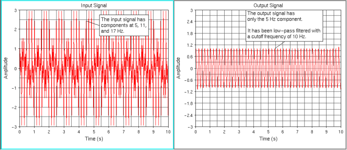
Filtering
A common practice in signal processing is to smooth data by eliminating
high-frequency components. This is done using a low-pass filter. It is called a
low-pass filter because it only keeps low-frequency components and eliminates high
frequency components. Thus, it only lets low-frequency components pass. Other types
of filters are high-pass, band-pass, and band-stop, or notch, filters.
In order to filter a signal, the application transforms the input data into the
frequency domain using an FFT. All unwanted frequency components are eliminated by
multiplying the FFT values at these frequencies by zero. The modified frequency
domain data is then transformed back into the time-domain.Figure 6. Low-Pass Filtered Signal
In order to specify which frequencies are to be removed, cutoff frequencies must be
defined. For low- and high-pass filters, only a single cutoff frequency is
necessary. For low-pass filters, frequencies below the cutoff frequency are passed,
while the opposite is true for high-pass filters. Band-pass and band-stop filters
require two cutoff frequencies, a low and a high. For a band-pass filter, only
frequencies between the two cutoff frequencies are passed, while for a band-stop
filter, only frequencies outside this range are passed.
One problem with this approach is that often the beginning and end of the filtered
signal do not match well with the original data. This is due to the fact that data
is missing on either side, making it more difficult to reconstruct the signal from
the filtered frequency data. Also, if the signal does not have a number of points
which are a valid number for an FFT, it will be zero-padded. In many cases, this
causes the filtered signal to sharply tend toward zero at the end. In order to
minimize this problem, often the input signal is concatenated with constant values
equal to the last value, then filtered, and finally the added values are
removed.
It is recommended that the mean be removed from a signal before it is filtered so the
mean of the filtered curve is 0.00. Then, add the mean back after filtering to
obtain the desired magnitudes. The mean may be left out altogether if the DC
component is not desired.
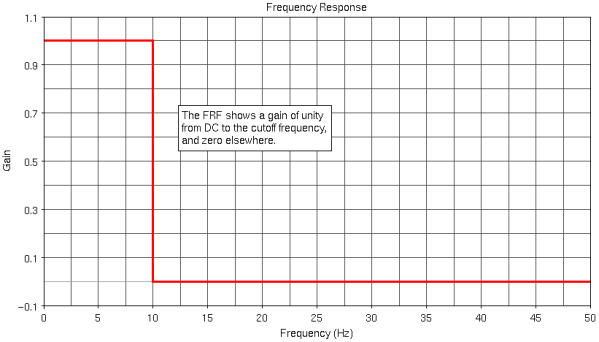
Frequency Response Functions
A Frequency Response Function, FRF, is used to determine the frequency
characteristics of a given system. The system must be quantified with an input
signal and an output signal.
The result of the FRF is a complex-valued function. Normally this is also shown in
magnitude/phase form. The magnitude spectrum gives information as to the system gain
at various frequencies, while the phase spectrum gives delay information.Figure 7.
For a system with a uniform gain and delay, the magnitude spectrum would be constant
at the gain of the system and the phase spectrum would be linear with slope
proportional to the system delay.
Blocking
Random data theoretically has no Fourier Transform, because it is aperiodic.
Therefore, in the Fourier Transform equation, , the upper
limit cannot be changed to the period of the signal. This would mean an infinite
amount of data would have to be collected in order to get the true Fourier Transform
of a random signal. In practice, this point is ignored. However, two random signals
from the same system will have vastly different spectral characteristics. In order
to circumvent this problem, a process known as blocking is often used.
In blocking, a single random signal is subdivided into many shorter signals. The
frequency characteristics of each of the smaller signals are calculated, and then
averaged. This takes advantage of a statistical property which states that if the
frequency spectra of a large enough number of signals are averaged, the results will
tend toward the true spectrum of the system.
However, by using this technique, the duration of each individual signal is lessened,
resulting in poorer frequency resolution. Since the sampling interval is the same
for each sub-signal as the original signal, the Nyquist frequency is not changed by
blocking.
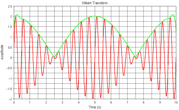
Hilbert Transform
The Hilbert Transform is used to obtain the envelope of a curve. It is in fact
guaranteed to be greater than or equal to the input signal for all data which is
functional, that is, the X values are monotonic or strictly increasing. It is done
using a complex algorithm incorporating FFTs. It tends to work very well with smooth
curves, but for noisy data the results are not as good. Also, as with
frequency-domain filtering, the beginning and end of the signal tend not to match
the original data very closely.Figure 8.