Processing math: 100%

What's New
View new features for Altair HyperWorks 2024.1.
Altair HyperWorks Introduction
Quick introduction to Altair HyperWorks products.
Tutorials
Discover the functionality of Altair HyperWorks products with interactive tutorials.
Altair HyperWorks Tools
Administrative tools to customize your Altair HyperWorks installation.
- Altair License Utility
  Use the Altair License Utility to determine a managed Altair Licensing ID, check license usage, borrow licenses, and set up managed Altair Units.
- Altair Compute Console
  Altair Compute Console (ACC) is a utility that allows you to start different Altair HyperWorks Solvers.
- Remote Job Submission
  Remote Job Submission in Altair Compute Console (ACC) is implemented as an alternative to a local run.
- Remote Server User Guide
- AbaqusODB Upgrade
  AbaqusODB UpGrade is a HyperView tool, which upgrades ODB files created in Abaqus 2018 (or earlier) to Abaqus 2023.
- HgTrans
  HgTrans translates solver results files from their native file format to Altair Binary Format (ABF). This can be done using the HgTrans GUI or via the HgTrans batch mode.
- HvTrans
  HvTrans is a result translator for HyperView that translates solver result files to .h3d files.
- HWTK GUI Toolkit
  The HWTK GUI Toolkit is a resource tool for coding Tcl/Tk dialogs. It contains documentation of the HWTK GUI Toolkit commands, demo pages that illustrate our Altair GUI standards, and sample code for creating those examples.
- Cleanup Utility
  The Cleanup Utility is a script for Windows that removes any custom settings that you may have due to the Altair applications installed.
- Model Identification Tool
  The Model Identification Tool (MIT) is a profile in HyperGraph for fitting test data from frequency- and amplitude-dependent bushings to analytical models. The MIT operates in conjunction with HyperGraph, MotionView and MotionSolve to provide you with a comprehensive solution for modeling and analysis.
  - MIT and the Fitting Process
  - Start MIT
    This section explains how to start the MIT interactively and in batch mode.
  - Use MIT
    This section explains how to use the features in HWTK GUI Toolkit.
  - Appendix I: SPD File Format Specification
  - Altair Bushing Model
    The Altair Bushing Model is a library of sophisticated, frequency- and amplitude-dependent bushing models that you can use for accurate vehicle dynamics, durability and NVH simulations. The Altair Bushing Model supports both rubber bushings and hydromounts.
  - Use the Altair Bushing Model with MotionView
    This section provides information about using the Altair Bushing Model, also known as AutoBushFD, with MotionView. The Altair Bushing Model is a sophisticated model that you can use to simulate the behavior of bushings in vehicle dynamics, durability and NVH simulations.
  - Use the Altair Bushing Model with MotionSolve
    This section provides information about using the Altair Bushing Model, also known as AutoBushFD, with MotionSolve.
    - Features of the Altair Bushing Model
    - Select Force Models in the Bushing Property File
    - Theory and Formulations
      - Stiffness Force Models
        The Altair Bushing Model includes Stiffness Force Models for Spline Stiffness, Constant Stiffness and Cubic Stiffness:
      - Damping Force Models
        The Altair Bushing Model includes the following Damping Force Models:
        Constant Damping Model
        Rubber Damping Model
        Schematic and Equations
        First Order Filter
        Scale Factors P0, P1, P2, and Q0, Q1, Q2
        Multiple Preloads
        Factor RMIN
        Select a Lower Bound of R and Rmin
        Hydromount Damping Model
      - Friction Formulation
        This section provides information about the LuGre and Dahl formulations for friction.
      - Mount Stiffness
        The bodies connected by the bushing are flexible and may deflect under the load being transmitted. This phenomenon is modeled with the Mount Stiffness feature. Mount stiffness models the structural stiffness of the bodies, thus mounting the bushing as a linear spring and damper in series with the bushing in each direction.
      - Mount Limits
        The Altair Bushing Model includes a Mount Limits feature, which lets you model the material contact that occurs between the bodies that a bushing connects. The bodies are flexible and may deflect under the load being transmitted. Given enough bushing deflection, the bodies may contact one another for negative and positive deflections in each direction.
      - Preload, Offset, and Scale
        This section describes how preloads, offsets and scales enter into bushing force computations. You use Preloads, Offsets and Scales to alter the operating point of a bushing. You can offset the bushing displacement in any direction, and scale the input displacement and velocity. You can also offset the bushing force in any direction by adding a preload or scale-output force or moment in any direction.
      - Coupling
        Coupling refers to the forces and moments generated in a bushing to oppose the overall deformation of the bushing. These forces and moments are independent of any coordinate system that might be used to measure the deformation or deformation velocity. Coupling is an important factor when the bushing characteristics are non-linear.
      - Validate Test Data in the SPD File
        The System Performance Data file, *.spd, contains the test data used for fitting a bushing. This data should be validated to ensure that it is physically meaningful. One test for physical consistency is that the dynamic stiffness at any amplitude of vibration must always be greater than the static stiffness at the same amplitude.
    - Bushing Property File
    - Mount Limits Property File
    - References
  - Supported Solvers
- Register HVPcontrol
  Register HVPcontrol registers the HVP ActiveX control for HyperView Player.
- HyperWorks Automation Toolkit
  The HyperWorks Automation Toolkit (HWAT) is a collection of functions and widgets that allows an application to quickly assemble HyperWorks automations with minimal effort and maximum portability.
- H3D Validation Tools
  The H3D Validation Tools available are H3D Info and H3D Validate.
- Uninstall
  Use the Altair HyperWorks Products Uninstaller to remove all files from the installation directory.

View All Altair HyperWorks Help

Schematic and Equations

This model can be used for both dynamic and quasi-static tests.

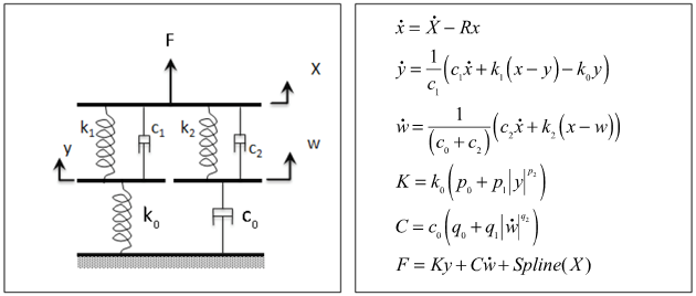
Figure 1.

The figure above-left shows a schematic of the bushing model where:

X is the input displacement provided to the bushing.
y and w are the internal states of the bushing.
$k_{0}$ and $k_{1}$ represent the bushing rubber stiffness.
$k_{2}$ is used to control the stiffness at large velocities.
$c_{0}$ produces the roll-off observed in the experimental data at low velocities.
$c_{1}$ accounts for the relaxation of the bushing impact force.
$c_{2}$ represents the viscous damping observed at large velocities.

The governing equations for this bushing are shown above-right where:

R is the cutoff frequency associated with a first order filter that acts on the input X.
x is the dynamic content of the bushing input X. This is the filter output.
$\dot{y}$ and $\dot{w}$ are the time derivatives of the internal states of the bushing y and w.
K is the effective stiffness of the bushing.
C is the effective damping of the bushing.
Spline (X) is the static force response of the bushing.

The effective stiffness K and effective damping C are dependent on nonlinear effects such as friction in the bushing material and other nonlinear behavior that cannot be easily represented physically.

The effective stiffness K is $k_{0}$ multiplied by a factor:
$S_{y} = (p_{0} + p_{1} {| y |}^{^{p_{2}}})$
Similarly, the effective damping C is $c_{0}$ multiplied by a factor:
$S_{w} = (q_{0} + q_{1} {| \dot{w} |}^{^{q_{2}}})$

The total force generated by the bushing is the sum of 2 forces:

Static force at the operating point: Spline (X)
Force due to the dynamic behavior of the bushing: $K y + C \dot{w}$