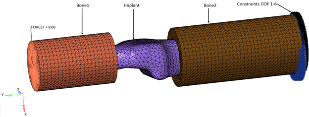
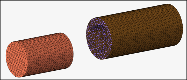
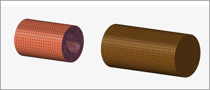
Figure 1 shows the
structural model used for this tutorial: A Hyperelastic Implant connected to bone on
both sides. A force of 9 Newtons is applied at one end of the model and the other
end of the model is constrained with all degrees of freedom.
The arthritic finger is modeled using hyperelastic material and subjected to a force
of 9 N, aiming to rotate the finger by 90 degrees. The results of strain,
displacement and stresses are analyzed for the TIE contact.
The following exercises are included:
Create Hyper Elastic material
Create Hyper Elastic property
Set up boundary conditions and imposed load
Define contact between implant and bones
Define nonlinear implicit parameters
Set up NLSTAT analysis
Submit job and view result
Launch HyperMesh
Launch HyperMesh.
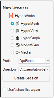
In the New Session window, select HyperMesh from the list of tools.
For Profile, select OptiStruct.
Click Create Session.
Figure 2. Create New Session This loads the user profile, including the appropriate template, menus,
and functionalities of HyperMesh relevant for
generating models for OptiStruct.
Import the Model
On the menu bar, select File > Import > Solver Deck.
In the Import File window, navigate to and select
Arthritis_Finger.fem you saved to your
working directory.
Click Open.
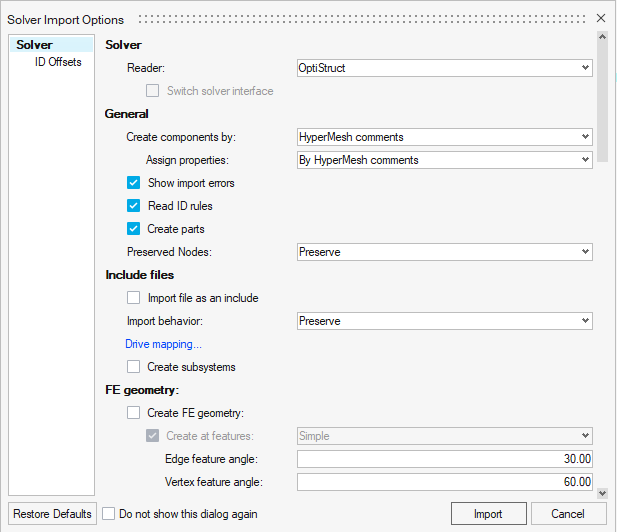
In the Solver Import Options dialog, ensure the Reader is
set to OptiStruct.
Figure 3. Import Base Model in HyperMesh
Accept the default settings and click Import.
Set Up the Model
Create Curves
In this step, create the curves for the hyper elastic material.
In the Model Browser, right-click and select
Create > Curve.
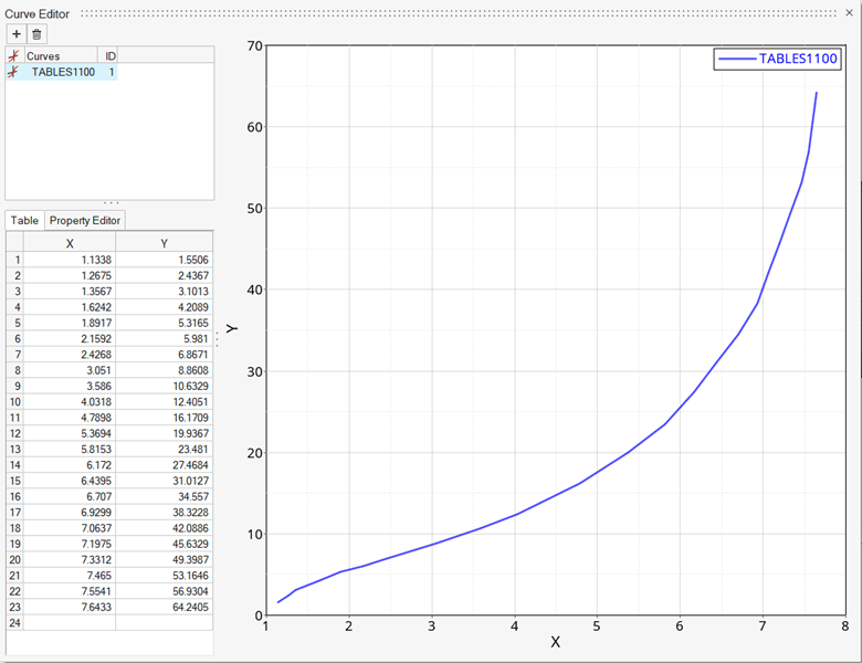
A default window for the Curve Editor
opens.
Right-click on the new table and select Rename.
For name, enter TABLES1100.
Enter the following values in the X and Y fields:
Table 1. Simple Tension Compression Data Values
X (stress)
Y (strain)
1.1338
1.5506
1.2675
2.4367
1.3567
3.1013
1.6242
4.2089
1.8917
5.3165
2.1592
5.981
2.4268
6.8671
3.051
8.8608
3.586
10.6329
4.0318
12.4051
4.7898
16.1709
5.3694
19.9367
5.8153
23.481
6.172
27.4684
6.4395
31.0127
6.707
34.557
6.9299
38.3228
7.0637
42.0886
7.1975
45.6329
7.3312
49.3987
7.465
53.1646
7.5541
56.9304
7.6433
64.2405
Figure 4.
Click Close.
In the Model Browser, double-click
Curves and select
TABLES1100.
For Card Image, select TABLES1 from the drop-down
menu.
Create another curve for equi-biaxial tension.
For Name, enter TABLES1200.
Enter the following values in the X and Y fields:
Table 2. Equi-biaxial Tension Data Values
X
Y
1.02
0.9384
1.06
1.59
1.11
2.4087
1.14
2.622
1.2
3.324
1.31
4.4278
1.42
5.183
1.68
6.6024
1.94
7.7794
2.49
9.7857
3.03
12.6351
3.43
14.6804
3.75
17.4
4.07
20.1058
4.26
22.4502
4.45
24.653
For Card Image, select TABLES1.
Create another curve for pure shear loading data.
For Name, enter TABLES1400.
Enter the following values in the X and Y fields:
Table 3. Pure Shear Loading Data Values
X
Y
1.069
0.6
1.1034
1.6
1.1724
2.4
1.2828
3.36
1.4276
4.2
1.8483
6
2.3862
7.8
3.0
9.6
3.4897
11.12
4.0345
12.96
4.4483
14.88
4.7793
16.58
5.0621
18.2
For Card Image, select TABLES1.
Create another curve for volumetric data.
For Name, enter TABLES1500.
Enter the following values in the X and Y fields:
Table 4. Volumetric Data Values
X
Y
0.9703
60
0.9412
118.2
0.9127
175.2
0.8847
231.1
For Card Image, select TABLES1.
Define the Hyper Elastic Implant Material
The hyper elastic behavior of the implant must be defined.
In the Model Browser, right-click and select
Create > Material.
For Name, enter Implant.
Click Color and
select a color from the color palette.
For Card Image, select MATHE from the drop-down
menu.
For MODEL, select ABOYCE from the drop-down menu.
For TAB1, select load-curve TABLES1100.
For TAB2, select load-curve TABLES1200.
For TAB4, select load-curve TABLES1400.
For TABD, select load-curve TABLES1500.
Define the Bone Material
In the Model Browser, right-click and select
Create > Material.
For Name, enter Bone.
Click Color and
select a color from the color palette.
For Card Image, select MAT1 from the drop-down
menu.
For E, enter 14800.
For NU, enter 0.3.
Define the Implant Property
In the Model Browser, right-click and select
Create > Property.
For Name, enter Implant.
Click Color and
select a color from the color palette.
For Card Image, select PSOLID from the drop-down
menu.
For Material, click Unspecified > Material.
In the dialog, select Implant from the list of materials
and click OK.
Define the Bone Property
In the Model Browser, right-click and select
Create > Property.
For Name, enter Bone.
Click Color and
select a color from the color palette.
For Card Image, select PSOLID from the drop-down
menu.
For Material, click Unspecified > Material.
In the dialog, select Bone from the list of materials
and click OK.
Define the Contact Interface Property
In the Model Browser, right-click and select
Create > Property.
For Name, enter PCONT.
Click Color and
select a color from the color palette.
For Card Image, select PCONT from the drop-down
menu.
Under STIFF_REAL_VAL, for STIFF, choose HARD from the
drop-down menu.
Under MU1 Options, for MU1, enter 0.3.
Assign Properties to Components
Assign the Implant property.
In the Component Browser, select Implant.
For Property, click Unspecified > Property and select Implant from the
list.
The Material field is auto-filled with Implant.
Click OK.
Assign the Bone1 property.
In the Component Browser, select Bone1.
For Property, click Unspecified > Property and select Bone from the
list.
The Material field is auto-filled with Bone.
Click OK.
Assign the Bone2 property.
In the Component Browser, select Bone2.
For Property, click Unspecified > Property and select Bone from the
list.
The Material field is auto-filled with Bone.
Click OK.
Define the Set Segment for the Implant
In the Component Browser, right-click on Implant and
select Isolate from the context menu.
In the Model Browser, click Create > Set Segment.
For Name, enter Implant.
Click Color and
select a color from the color palette.
For Card Image, select SURF from the drop-down
menu.
For Elements, select 0 Elements > Elements.
In the drop-down menu, select faces.
Select all faces of the Implant component in the modeling window.
Define the Set Segment for the Bone
In the Component Browser, right-click on Bone1 and
Bone2 and select Isolate from
the context menu.
In the Model Browser, click Create > Set Segment.
For Name, enter Bone.
Click Color and
select a color from the color palette.
For Card Image, select SURF from the drop-down
menu.
For Elements, select 0 Elements > Elements.
In the drop-down menu, select faces.
Select all inside faces of the Bone1 and Bone2 components in the modeling window.
Figure 5. Figure 6.
Define TIE Contact
In the Model Browser, right-click and select
Create > Contact.
For Name, enter Tie_Contact.
Click Color and
select a color from the color palette.
For Card Image, select TIE from the drop-down
menu.
For Secondary Entity IDs, click Unspecified > Set Segment and select Implant.
For Main Entity IDs, click Unspecified > Set Segment and select Bone.
For DISCRET, select N2S from the drop-down menu.
Apply Loads and Boundary Conditions
Define Nonlinear Implicit Parameters
In the Model Browser, right-click and select
Create > Load Step Inputs.
A default load step input editor window opens.
For Name, enter NLPARM.
For Config Type, select Nonlinear Parameters from the
drop-down menu.
By default, for Type NLPARM is selected.
Define NLADAPT Load Step Inputs
In the Model Browser, right-click and select
Create > Load Step Inputs.
A default load step input editor window opens.
For Name, enter NLADAPT.
For Config Type, select Time step Parameters from the
drop-down menu.
By default, for Type NLADAPT is selected.
Select the NCUTS check box and enter a value of
25 in the text box.
Define NLMON Load Step Inputs
In the Model Browser, right-click and select
Create > Load Step Inputs.
A default load step input editor window opens.
For Name, enter NLMON.
For Config Type, select Runtime Monitoring from the
drop-down menu.
By default, for Type NLMON is selected.
For ITEM, select DISP from the drop-down menu.
For INT, select ITER from the drop-down menu.
Define NLOUT Load Step Inputs
In the Model Browser, right-click and select
Create > Load Step Inputs.
A default load step input editor window opens.
For Name, enter NLOUT.
For Config Type, select Output Parameters from the
drop-down menu.
By default, for Type NLOUT is selected.
For Nonlinear Incremental Output, select NINT from the
drop-down menu.
For VALUE, enter 10.
Select the SVNONCNV check box and for VALUE, select
YES.
Define the CNTSTB Load Collector
In the Model Browser, right-click and select
Create > Load Collector.
For Name, enter CNTSTB.
Click Color and
select a color from the color palette.
For Card Image, select CNTSTB from the drop-down
menu.
For S0, enter 0.01.
For S1, enter 1e-05.
Define the Boundary Condition SPC
In the Model Browser, right-click and select
Create > Load Collector.
For Name, enter spc.
Click Color and
select a color from the color palette.
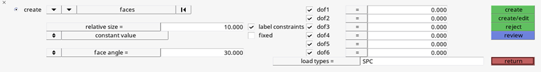
Open the Analyze ribbon and select BCs > Constraints.
A panel to define the constraint opens.
On the first drop-down menu in the panel, select
nodes.
On the second drop-down menu, select faces.
In the modeling window, select the entire rear side
face (all nodes) of Bone1.
For load types, select SPC.
Select all dof check boxes and enter
0.0 in the corresponding text boxes.
Figure 7. Figure 8.
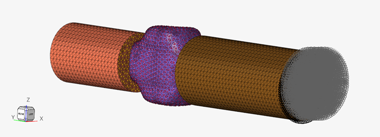
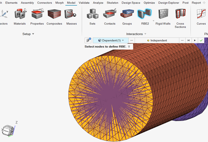
Define Force
In the Model Browser, right-click and select
Create > Component.
For Name, enter RBE2.
Click Color and
select a color from the color palette.
On the guide bar, select Dependent and choose
faces from the drop-down menu.
Select the front face of Bone2 and click .
Figure 9. Face Selection for RBE2
In the Model Browser, click Create > Load Collector.
For Name, enter Force.
Click Color and
select a color from the color palette.
Select the Analyze ribbon.
On the Loads tool, select the Forces sub tool.
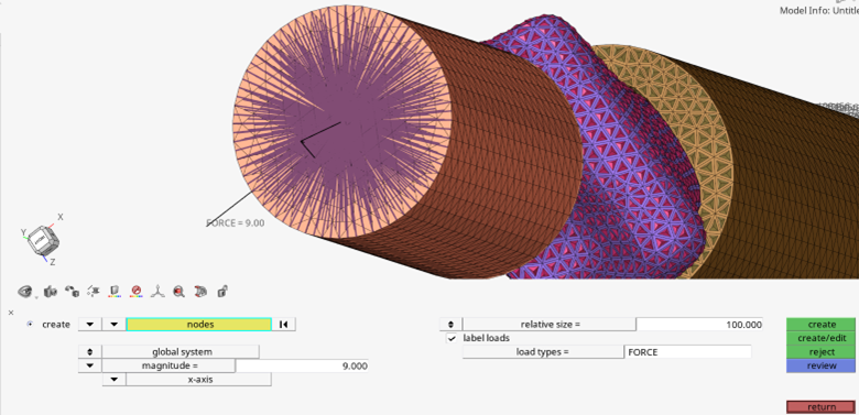
Figure 10. The corresponding panel opens.
In the modeling window, select the center node of
RBE2.
For magnitude, enter 9.0.
From the drop-down menu below magnitude, select
x-axis.
For load types, select FORCE.
Figure 11. Force Load RBE2
Define Output Control Parameters
Select the Analyze ribbon.
On the drop-down menu for the Run tool group, select Control
Cards.
On the Control Cards panel, select
GLOBAL_OUTPUT_REQUEST.
For all selected output parameters (ELFORCE,
SPCF, STRAIN,
STRESS), for FORMAT(1), select
H3D.
Save the Database
Click File > Save.
For File Name, enter Arthritis_Finger.hm.
Click Save.
Run the Analysis
Select the Analyze ribbon.
In the Run tool group, select Run OptiStruct
Solver.
Click save as.
In the Save As dialog, specify location to write the
OptiStruct model file and enter
Arthritis_Finger for filename.
For OptiStruct input decks,
.fem is the recommended extension.
Click Save.
The input file field displays the filename and location specified in the
Save As dialog.
Set the export options toggle to all.
Set the run options toggle to analysis.
Set the memory options toggle to memory default.
Click OptiStruct to run the analysis.
If the job was successful, new files are available in the directory
where you chose to write the files. OptiStruct also
reports error messages if any exist. The file Arthritis_Finger.out can be opened in a text editor to
find details regarding any errors. This file is written to the same directory as
the .fem file.
View the Results
In the Solver window, select Results to open the results
in HyperView.
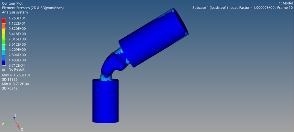
HyperView, select Contour.
For Results Type, in the first drop-down menu, select Element
Stresses (2D & 3D) (t).
For Results Type, in the second drop-down menu, select
vonMises.
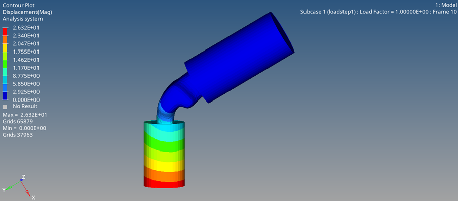
Figure 12. Contour of Element Stresses in Bone and Implant Subject to
Loading Figure 13. Contour of Displacement in Bone and Implant Subject to
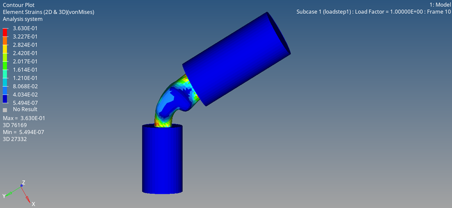
Loading Figure 14. Contour of Element Strains in Bone and Implant Subject to
Loading

 .
.
 .
.