HL-T: 1010 Uniaxial Strain-Life (E-N)
In this tutorial you will:
- Import a model to HyperLife
- Select the EN module and define its required parameters
- Create and assign a material
- Assign load histories for scaling the stresses from FEA subcases
- Evaluate and view results
Import the Model
-
From the Home tools, Files tool group, click the Open Model tool.
Figure 1. 
-
From the Load model and result dialog, browse and select
HL-1010\Hook.h3d for the model
file.
The Load Result field is automatically populated. For this tutorial, the same file is used for both the model and the result.
-
Click Apply.
Figure 2. 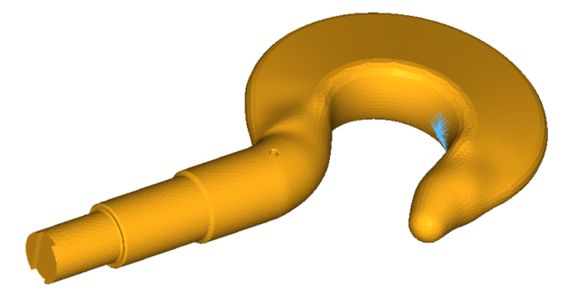
Tip: Quickly import the model by dragging and
dropping the .h3d file from
a windows browser into the HyperLife
modeling window.
Define the Fatigue Module
-
Click the arrow next to the fatigue module icon and select the
EN tool from the list of options.
Figure 3. 
The EN dialog opens. -
Define the EN configuration parameters.
- Select Uni Axial as the method.
- Select MPa for the FE model units.
- Select Signed von for the stress combination.
- Enter a value of 0.5 for the certainty of survival.
- Select SWT for the mean stress correction.
- Select NEUBER for the plasticity stress connection.
- Select Worst for the layer selection.
- Select Time Series for the type of loading.
Figure 4. 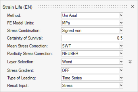
- Exit the dialog.
Assign Materials
-
Click the Material tool.
Figure 5. 
The Assign Material dialog opens. - Activate the checkbox next to the part HOOK_solid.
- Click the My Material tab.
-
Click
 .
A new material named Mat_EN("n") is created.
.
A new material named Mat_EN("n") is created. - Set the Elastic Modulus to 70000.
- Set the Standard Error of Log(elastic strain) (SEe) to 0.0.
- Set the Standard Error of Log(plastic strain) (SEp) to 0.0.
-
Click Plot & Save.
Figure 6. 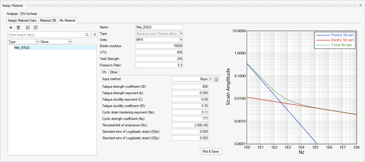
- Right-click on the newly created material and select Add to Assign Material List.
- Click the Assign Material Data tab.
-
For HOOK_solid, select Mat_EN("n") from the Material
drop-down menu.
Tip: Preview the EN plot by clicking
 .
. -
Accept the default parameters in the Assign Material Data tab.
Figure 7. 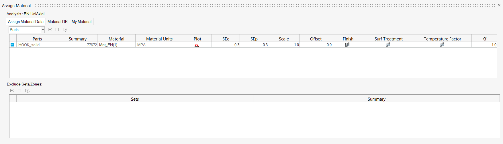
- Exit the dialog.
Assign Load Histories
-
Click the Load Map tool.
Figure 8. 
The Load Map dialog opens. - From the Channel Type drop-down menu at the top of the dialog, select Time Data.
-
Click
 in the Choose File
field and browse for load1.csv.
in the Choose File
field and browse for load1.csv.
-
Click to
add the load case.
- Optional:
Click to view a plot of
the load.
Figure 9. 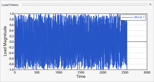
Tip: Expand the width of the dialog to view a clearer picture of the plot. - On the bottom half of the dialog, verify Auto is selected for event creation.
-
Select Subcase 1 and Subcase 2,
then click to create an
event.
- For Configuration, select Superposition.
- Select and drag-and-drop the load 1 (block1) channel into the Channels column of the event.
- Right-click the newly added Block 1 <load1> channel, and select Apply value to current event from the context menu.
- For Repeats, enter 100.
- For Subcase 1, enter 5 for Scale.
-
Activate the Event_1 checkbox.
Figure 10. 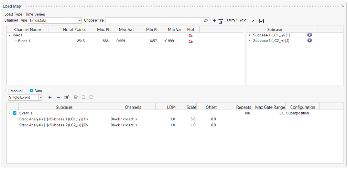
- Exit the dialog.
Evaluate and View Results
-
From the Evaluate tool group, click the
Run Analysis tool.
Figure 11. 
The Evaluate dialog opens.Figure 12. 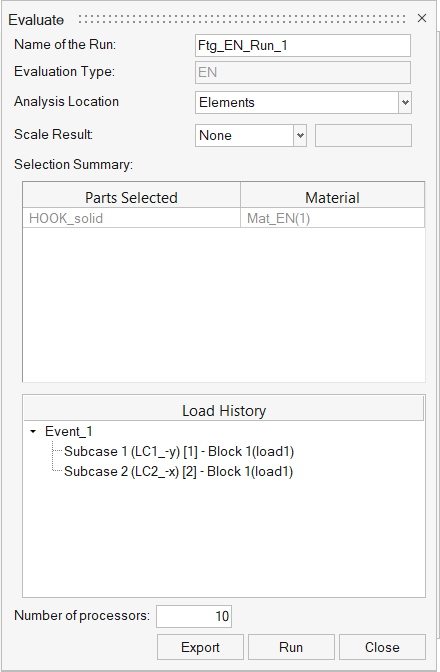
- Optional: Enter a name for the run.
-
Click Run.
Result files are saved to the home directory and the Run Status dialog opens.
- Once the run is complete, click View Current Results.
-
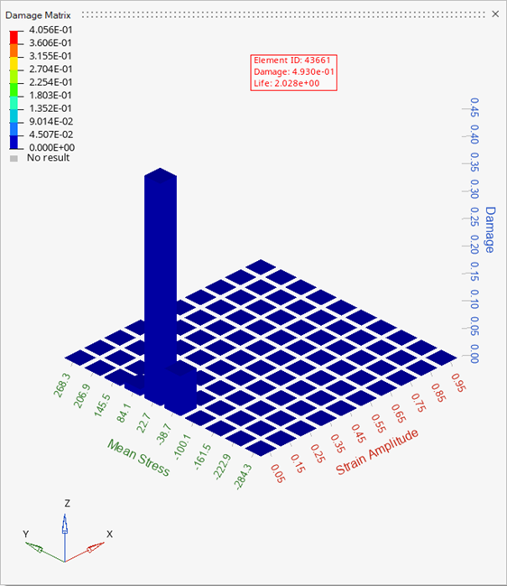
Use the Results Explorer to
visualize various types of results.
Figure 13. 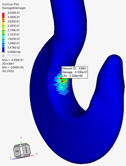
Figure 14.