Use Plots to View Grid Participation

Create and view contour plots by selecting various scales, grids, and grid IDs for the specified Structure or Fluid grid participation.

Load Files and Select Result Options

From the NVH-Utilities > Grid Participation tab, click the Load sub-tab.

Under File selection, use the file browsers to select the file(s) that you would like to load.

Option	Description
Result	Select the result file using the file browser (.h3d, .pch, .res, or .op2). Attention: A PCH file cannot be read directly into HyperView, therefore it has to be converted into the RES format. The translation process includes running a special version of HMNast to convert the PCH file into the RES file, which is then used for plotting.
Cavity	Select the model file which contains the solid elements for the cavity (.fem, .dat, or .bdf). Note: This file is not required if an OptiStruct .h3d or Nastran (MSC) .op2 file is loaded into the Result file field.
Structure	Select the model file which contains the solid elements for the structure (.fem, .dat, or .bdf). Note: This file is not required if an OptiStruct .h3d or Nastran (MSC) .op2 file is loaded into the Result file field.
Interface	Select the model file which contains the elements on the interface of the cavity and structure interaction (.interface). Note: This file is not required if an OptiStruct .h3d or Nastran (MSC) .op2 file is loaded into the Result file field.

Click the Load button to load the files designated in the File selection section of the tab.
Upon reading the file, the Result selection fields are populated (see below).

Under Result selection, select the options that will be used to investigate the participations.

Option	Description
H3D output	The H3D output option. Contour = Yes The grid participation results are output in a format that is ready for contouring (which reduces the amount of processing required for HyperView). Contour = No The grid participation results are output in a raw, unprocessed format.
Subcase	Displays the various subcases and their scale types available for selection from the drop-down menu - (s) indicates a scalar-type result, (c) indicates complex results, (t) indicates a tensor-type result, and (v) indicates a vector-type result. Note: There is a Fluid Grid ID raw data result type generated by OptiStruct which can also be viewed by using the various options in the Contour panel.
Response ID	Grid ID of the response for which Grid participation results are available. Select one from the drop-down menu.
Response label (optional)	Enter a label that describes the response, for example `"Driver’s Ear"`.
Result set	Select either a Structure Grid Participation plot or a Fluid Grid Participation plot.

Click the Display Options button to customize the plot, including scale, weighting, and the plot layout.
The Display Options dialog is displayed.
Click the Load Response button to apply the grid participation plot in the modeling window.
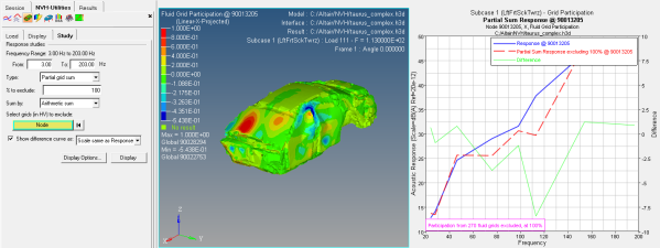
Figure 1. A Response Study Example

The response study is meant to accomplish two goals:
1. Find the upper limit of the selected nodes’ impact on the response. If it is too small, you may decide not to bother with optimizing the local structure there.
2. Identify the impact of the selected nodes over the entire frequency range analyzed. This is beneficial because it is often the case in solving NVH problems that improvement in one frequency is accompanied by degradations at others. Therefore, knowing the impact over the whole frequency ranges helps you to ensure that the solution created by modifying the structure at the selected nodes is a good overall solution.
See the HyperGraph User's Guide for additional information on plotting.

Display a Grid Participation Contour Plot

From the NVH-Utilities tab, click the Display sub-tab.

Note: To activate this tab, you must first load a file from the Load tab.

Select an option from the Direction component drop-down menu.

Option	Description
X	Grid participation results from the X component of grid vibration.
Y	Grid participation results from the Y component of grid vibration.
Z	Grid participation results from the Z component of grid vibration.
Sum of XYZ	Arithmetic sum of the grid participation results from the X, Y, and Z components of grid vibration.

Select an option from the Complex component drop-down menu.

Option	Description
Projected	Complex grid participation results are first projected to the response, and the resulting scalar values are then contoured.
Real	Real parts of the complex grid participation results are contoured.
Imaginary	Imaginary parts of the complex grid participation results are contoured.
Magnitude	The magnitudes of the complex grid participation results are contoured.
Phase	The phases of the complex grid participation results are contoured.

Select an option from the Frequency option drop-down menu.

Option	Description
Specific frequency	Select a specific frequency to contour grid participation results.
Sum of frequencies	Select multiple frequencies and sum the results corresponding to these frequencies to generate one contour plot.

Select an option from the Sum by option drop-down menu.

Option	Description
Arithmetic	Select how grid participation results from different frequencies are to be summed together to generate one contour plot.

Select an option from the Frequency weighting option drop-down menu.

Option	Description
A	Use to scale sum grid participation results from different frequencies. 'A weighting' is used to define equal loudness sound pressure levels.
Equal	Use to sum grid participation results from different frequencies.

Select frequencies from the Frequency List which will be included in the sum response.

Tip: Use the Display All, Display None, or Reverse Display buttons (located on the right side of the list) to quickly select/deselect frequencies.
Click the Display Options button to customize the plot, including scale, weighting, and the plot layout.
The Display Options dialog is displayed.
Once the result selection options and display options are complete, click Display to apply the fluid or structure grid participation contour plot to the model.
This will allow you to look for the particular area of the structure which has the most positive (in-phase) contributions and also the area that has the most negative (out-of-phase) contributions. You can then effectively reduce the acoustic response at a grid point by reducing the vibration/contribution coming from the positive/in-phase area, or by increasing the vibration/response in the negative contribution area.
In addition, you can also view and move through the various frequencies from the grid participations (in order to determine the positive and negative contributions) by clicking on the various frequencies located in the Frequency List.
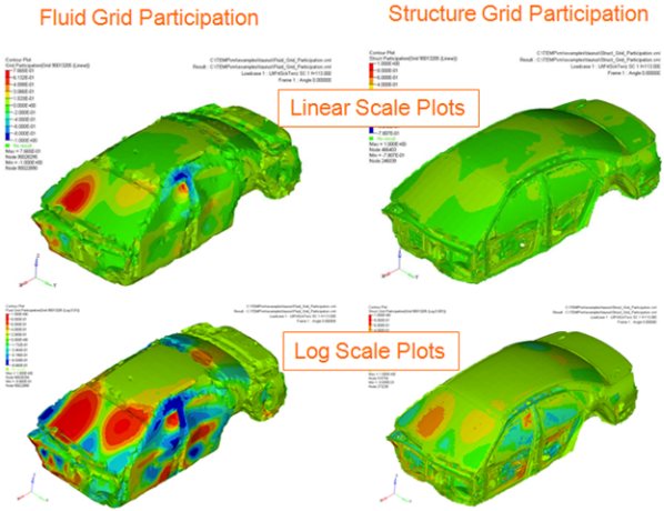
You can then apply additional fluid or structure grid plots, using log or linear or linear scale types, in order to isolate the most significant areas (see the example below):
Figure 2. The change in vibration results in reduced Structure participation and Fluid participation

Perform a Partial Grid Sum or Phaseless Sum Response Study

From the NVH-Utilities tab, click the Study sub-tab.

Note: To enable this option, you must first load a grid participation contour plot.
Under Response studies, enter in your custom frequency band in the Frequency Range: 3.00 Hz to 203.00 Hz From and To fields.
The frequency indicates the available range, based on the file loaded.

Select the type of response study from the Type drop-down menu.

Option	Description
Partial grid sum	Select a number of grids to exclude from the partial sum response, with an optional percentage to exclude.
Phaseless sum	Participation results from various grids are summed based on the magnitude only (without considering phase). Normally, both magnitude and phase are taken into consideration when grid participations are summed to calculate the response.

Optional: In the % to exclude field, enter the percentage of the contributors that you would like to exclude from the response.

Select an option from the Sum by drop-down menu.

Option	Description
Arithmetic sum	Participation results from various grids are summed based on the arithmetic sum of the complex grid participation.
Magnitude RSS	Participation results from various grids are summed based on the root sum of squares of the magnitude of the complex grid participation.

Under Select grids to exclude, select the grid that you would like to exclude from the response study by selecting nodes.
- Click the Node input collector and use the Extended Entity Selection Menu to select nodes.
- Activate the Node input collector and pick an nodes directly from the model in the modeling window.
The model is animated with respect to the selected entity. A new node can be defined and tracked at any time during animation by picking different nodes in the modeling window.

Select an option from the Show difference curve as drop-down menu.

Option	Description
% of Response	Plot the difference curve using a percentage of response scale and a new axis on the right hand side of the plot.
Scale same as Response	Plot the difference curve using the same scale as the one used to plot the response and a new axis on the right hand side of the plot.

Click the Display Options button to customize the plot, including scale, weighting, and the plot layout in the Display Options dialog.
Once your selections are complete, click Display to display the response study plot.

Note: See the HyperGraph User's Guide for additional information.

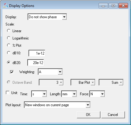
Grid Participation - Display Options Dialog

The Display Options dialog allows you to customize the response plot using various display and scaling options.

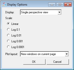
Figure 3. Load Tab and Study Tab - Display Options Dialog

Figure 4. Display Tab - Display Options Dialog

The following options are available:


Display	The following options are available from the Display drop-down menu:
	Do not show phase	Hides the phase values on the plot.
	Show phase	Displays the phase values on the plot.
	Single perspective view Attention: Available for the Display Tab only.	Displays a contour plot using only the isometric perspective.
	Multiple perspective view Attention: Available for the Display Tab only.	Displays multiple contour plots using the isometric, top, and bottom perspectives.
Scale	Displays the scale types available. Be sure to review the various scaling types in order to determine which type gives you the best spatial location of the contributions. For example, the Linear scale type is not very useful when looking at a Structure grid participation (the very localized red contributions displayed on the model) because it makes it extremely difficult to see the contributions. In many instances this contribution can be concentrated at one single point, and if there is only one grid contributing, then you essentially will not be seeing a very clear picture of where it is contributing. If that is the case, you will need to use another kind of scaling in order to make the area larger so that you will actually see a patch of the surface that contributes. You therefore want to find a scaling type which localizes the contribution without making the area too small to easily locate. Note: The Log extreme scaling versions are available for review (essentially everything on the model is displayed in red or blue); however these results are usually not very useful because they show that everything is equally effective in fixing the problem.
	Linear	Plots the linear values.
	Logarithmic	Plots the values in logarithmic scale. With this scale, data points are spread out more, which makes it easier to view.
	Log 0.1 Attention: Available for the Display Tab only.	Logarithmic scale with a reference value of 0.1.
	Log 0.01 Attention: Available for the Display Tab only.	Logarithmic scale with a reference value of 0.01.
	Log 0.001 Attention: Available for the Display Tab only.	Logarithmic scale with a reference value of 0.001.
	Log 0.0001 Attention: Available for the Display Tab only.	Logarithmic scale with a reference value of 0.0001.
	% Plot	Plots the contribution of the selected modes as a percentage of the total response. Percentage plot is a good option to use when comparing contributors versus the total response.
	dB10	10 logarithmic of the participation value over the reference value.
	dB20	20 logarithmic of the participation value over the reference value. For acoustic responses, the reference pressure is 20E-12 MPa.
	Weighting	Select a weighting option from the drop-down menu: A B C U A, B, C, and U-weighting are used to define equal loudness sound pressure levels.
	Unit	Activate the Unit check box and make selections from the following drop-down menus: Time (s, ms) Length (mm, m, ft, km, mile, inch) Force (N, KN, lbf)
Plot Layout	Select how the plot window will appear.
	New windows on current page	Plot is placed into a new window on the current page.
	Active window	Plot is placed into the active window.
	New windows on new page	Plot is placed into a new window on a new page.