In this tutorial, you will learn how to create waterfall plots.
From the 3D Chart ribbon, click the Waterfall
tool.Figure 1.
The Waterfall panel allows you to create waterfall plots from XY force response data
and input pulses. If a waterfall plot exists in the current window, the application
automatically fills in the default values.
Open the Session File and Create a 3D Chart Window
From the menu bar, select File > Session > Open.
From the 3dplotting folder, select the file trimmer.mvw
and click Open.
Click Close on the message log that appears.
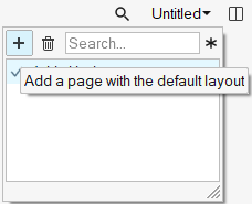
Create a page using the page navigation tools in the upper right corner.
Figure 2.
In the new window, click the Change Type icon () above the plot window and select 3D
Chart.
Create a Frequency versus Time Waterfall Plot
From the 3D Chart ribbon, click the Waterfall
tool.
Figure 3.
Verify that Frequency and Time are the options set under Plot Type.
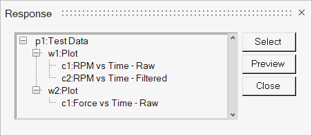
Click the curve selection icon in the Response Field for Data Curves:.
Choose the Force vs Time - Raw curve.
Figure 4.
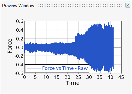
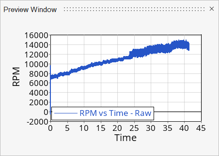
Click Preview to view the curve.
Figure 5.
Click Select.
Verify that the curve referenced under Response is p1w2c1.
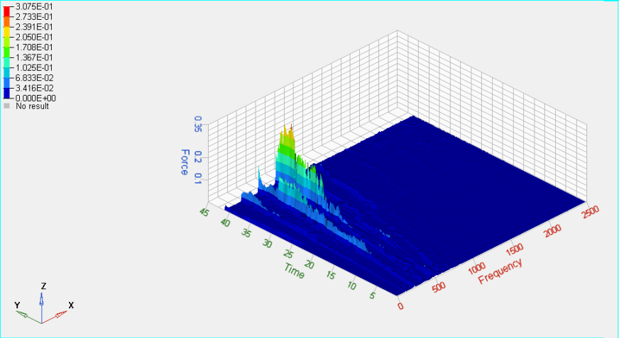
Enter 100 for Number under Waterfall slices.
Check the Contour waterfall option.
Click Apply.
Figure 6.
Create a Frequency versus RPM Waterfall Plot
While in the Waterfall panel, do the following:
For Plot Type: select Input Magnitude instead of Time
from the pull down menu.
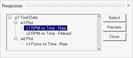
Under Data Curves, select RPM vs Time – Raw for
Response.
Figure 7. Figure 8.
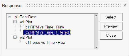
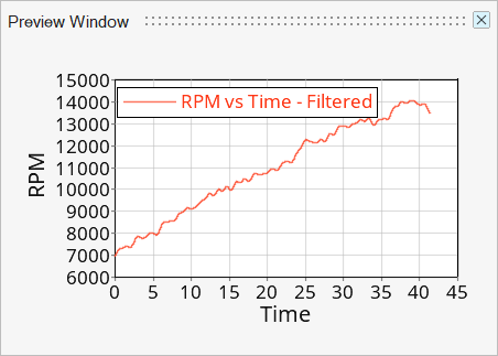
Select RPM vs Time – Filtered for Input under Data
Curves.
Figure 9. Figure 10.
Check the box for Input vector is in RPM to scale the
RPM to RPS.
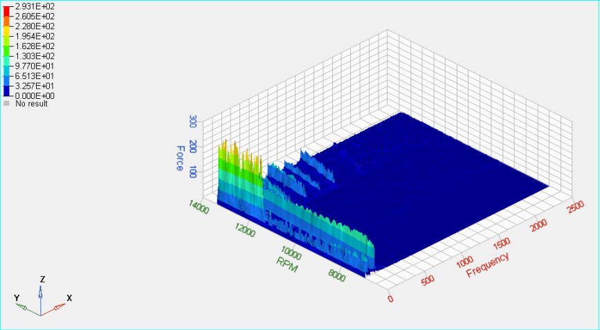
Click Apply.
Figure 11.
Click Undo to return to the Frequency vs Time
plot.
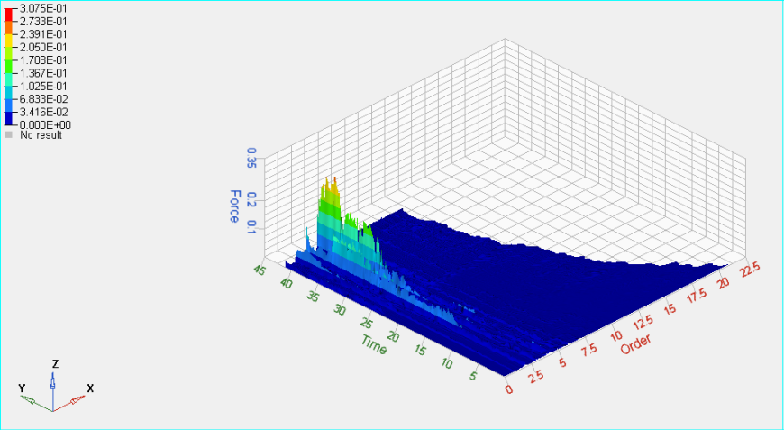
Create an Order Waterfall Plot
While in the Waterfall panel, do the following:
For Plot Type: select Order(scaled) instead of Frequency
from the pull down menu.
Select RPM vs Time – Filtered for Input under Data
Curves.
Click Apply to create the plot.
Figure 12.
Click Undo to return to the Frequency vs Time
plot.

 ) above the plot window and select 3D
Chart.
) above the plot window and select 3D
Chart.
 in the Response Field for Data Curves:.