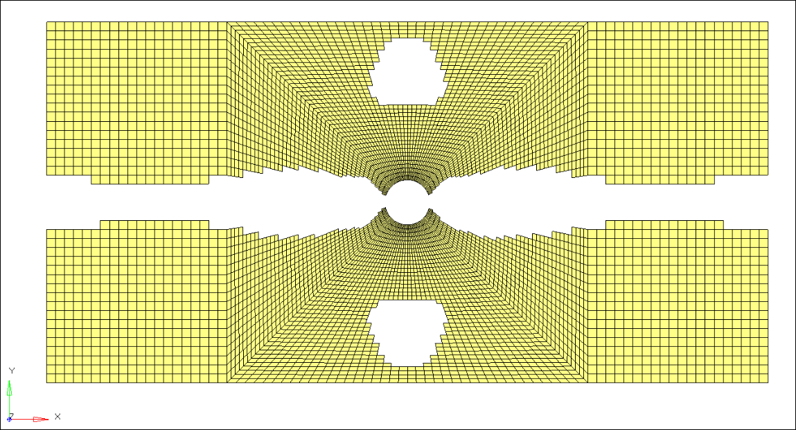
Phase 1:参照設計合成(フリー寸法最適化)
このフェーズでは、最適化セットアップを定義し、与えられた材料割合でもっとも剛性の高い設計を求めます。
フリー寸法最適化では、設計可能な各要素の板厚が設計変数として定義されます。この概念の複合材への適用は、設計変数が要素ごとの各‘スーパープライ’の板厚(同一プライ方向の全設計可能板厚)であることを意味します。
より理にかなった結果を得るには、製造姓制約条件を組み込み、すべての設計フェーズを通して自動的に適用します。
- 目標
- 荷重ケースのコンプライアンスを最小化
- 制約条件
- 体積率 < 0.3
- 設計変数
- 各プライ方向の要素板厚
- 製造性制約条件
- 0°のプライパーセンテージは80%以下存在
最適化のセットアップ
フリー寸法最適化設計変数の作成
- Analysisページからパネルoptimizationをクリックします。
- free sizeパネルをクリックします。
-
フリー寸法最適化の設計変数を作成します。
- createサブパネルを選択します。
- desvar=欄にfree-sizeと入力します。
- typeをSTACKにセットします。
- 積層板セレクターを使って、laminateを選択します。
- createをクリックします。
図 1. free-sizeパネルの欄への入力 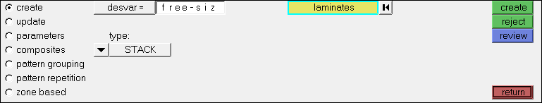
- compositesサブパネルを選択します。
- desvar=欄をクリックしてfree-sizeを選択します。
-
editをクリックします。
DSIZEパネルが開きます。このパネルでは、プライパーセンテージ、プライバランスおよびプライの減少についての製造性制約条件を定義します。
-
PLYPCTを定義します。
これらの値は、設計空間内の任意の要素について、0および90度のプライを、積層版の全板厚の20%から70%の間に制約します。
図 2. PLYPCTカードのDSIZEデータエントリ欄 
-
BALANCEを定義します。
図 3. BALANCEカードのDSIZEデータエントリ欄 
-
PLYDRPを定義します。
図 4. PLYSLP法を使ったPLYDRPカードのDSIZEデータエントリ欄 
- returnをクリックし、compositesサブパネルに戻ります。
- updateをクリックします。
- returnをクリックし、Optimization panelに戻ります。
Create Optimization Responses
- From the Analysis page, click optimization.
- Click Responses.
-
Create the volume fraction response.
- In the responses= field, enter Volfrac.
- Below response type, select volumefrac.
- Set regional selection to total and no regionid.
- Click create.
-
Create the compliance response.
- In the response= field, enter compliance.
- Below response type, select compliance.
- Set regional selection to total and no regionid.
- Click create.
- Click return to go back to the Optimization panel.
Create Design Constraints
- Click the dconstraints panel.
- In the constraint= field, enter volfrac.
- Click response = and select volfrac.
- Check the box next to upper bound, then enter 0.3.
- Click create.
- Click return to go back to the Optimization panel.
Define the Objective Function
- Click the objective panel.
- Verify that min is selected.
- Click response= and select compliance.
- Using the loadsteps selector, select nx_step.
- Click create.
- Click return twice to exit the Optimization panel.
出力リクエストの作成
- Analysisページからcontrol cardsパネルを選択します。
- Card Imageダイアログで、OUTPUTをクリックします。
- number_of_outputsに3と入力します。
-
3番目の行で、KEYWORDをFSTOSZに、FREQをYESに設定します。
このキーワードで、OptiStructはフリー寸法最適化後のサイジングモデルを自動的に生成します。
図 5. Phase 2についてfree-size to size(FSTOSZ)最適化出力ファイルをリクエスト 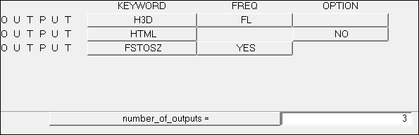
- returnを2回クリックし、Analysisページに戻ります。
データベースの保存
- menu barでをクリックします。
- Save Asダイアログでファイル名欄にoht_opti_ph1.hmと入力し、自身の作業ディレクトリに保存します。
Run the Optimization
- From the Analysis page, click OptiStruct.
- Click save as.
-
In the Save As dialog, specify location to write the
OptiStruct model file and enter
oht_opti_ph1 for filename.
For OptiStruct input decks, .fem is the recommended extension.
-
Click Save.
The input file field displays the filename and location specified in the Save As dialog.
- Set the export options toggle to all.
- Set the run options toggle to optimization.
- Set the memory options toggle to memory default.
-
Click OptiStruct to run the optimization.
The following message appears in the window at the completion of the job:
OPTIMIZATION HAS CONVERGED.
FEASIBLE DESIGN (ALL CONSTRAINTS SATISFIED).
OptiStruct also reports error messages if any exist. The file oht_opti_ph1.out can be opened in a text editor to find details regarding any errors. This file is written to the same directory as the .fem file. - Click Close.
The default files that get written to your run directory include:
- oht_opti_ph1.out
- OptiStruct output file containing specific information on the file setup, the setup of the optimization problem, estimates for the amount of RAM and disk space required for the run, information for all optimization iterations, and compute time information. Review this file for warnings and errors that are flagged from processing the oht_opti_ph1.fem file.
- oht_opti_ph1_des.h3d
- HyperView binary results file that contain optimization results.
- oht_opti_ph1_s#.h3d
- HyperView binary results file that contains from linear static analysis, and so on.
- oht_opti_ph1_sizing.*.fem
- A ply-based sizing optimization input file generated during free-sizing phase. This resulting deck contains PCOMPP, STACK, PLY, and SET cards describing the ply-based composite model, as well as DCOMP, DESVAR, and DVPREL cards defining the optimization data. The * sign represents the final iteration number.
- oht_opti_ph1_sizing.*.inc
- An ASCII include file contains the same ply-based modeling and optimization data as in the input deck. The * sign represents the final iteration number.
結果の表示
要素板厚結果の表示
-
OptiStructパネルから、HyperViewをクリックします。
HyperViewが起動し、2つのH3Dファイルからの結果が含まれた3つのページを含むセッションファイルoht_opti_ph1.mvwが開きます。
- Page 2
- oht_opti_ph1_des.h3d内の最適化結果。
- Page 3
- oht_opti_ph1_s1.h3d内のsubcase 1の解析結果。
注: これらのファイルをスタンドアローン版のHyperMeshから開く際は、ページ番号が小さくなります。 - oht_opti_ph1_des.h3dの結果を含むページに進みます。
-
Resultsツールバーで
 をクリックし、Contour panelを開きます。
-
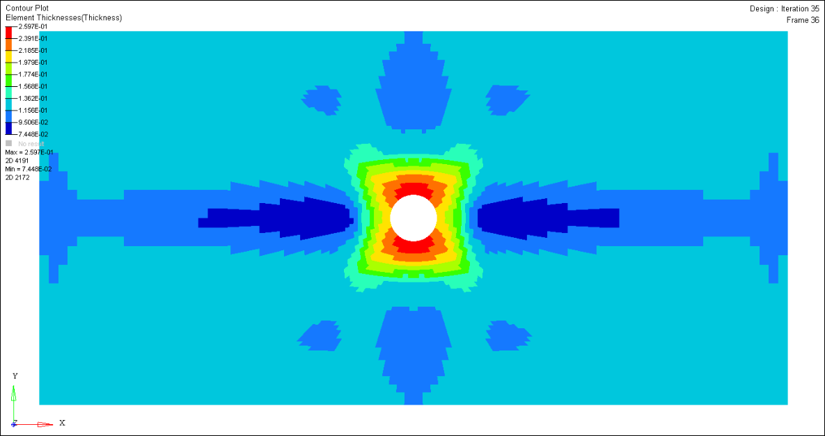
プロットオプションを選択します。
図 6. Contour panelのプロットオプション(フリー寸法最適化結果) 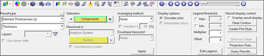
-
Results Browserから、最終反復計算を選択します。
図 7. 最終反復計算の選択 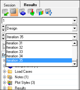
- Applyをクリックします。
-
Standard Viewsツールバーで
 をクリックし、X-Yプレーンで結果を確認します。
プライ板厚結果の表示
- Contour panelで、Result typeを Ply Thicknesses (s)に設定してください。
-
プロットオプションを選択します。
図 9. プライ板厚のコンタープロット 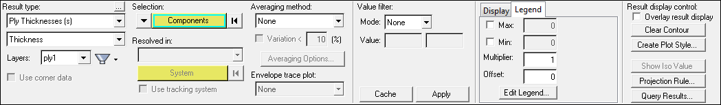
- Results Browserから、最終反復計算を選択します。
-
Applyをクリックします。
0度のスーパープライの板厚分布が生成されます。これは、0°のプライバンドルのプライ形状とパッチ位置を表すものです。
図 10. 0度のスーパープライのプライ板厚コンタープロット 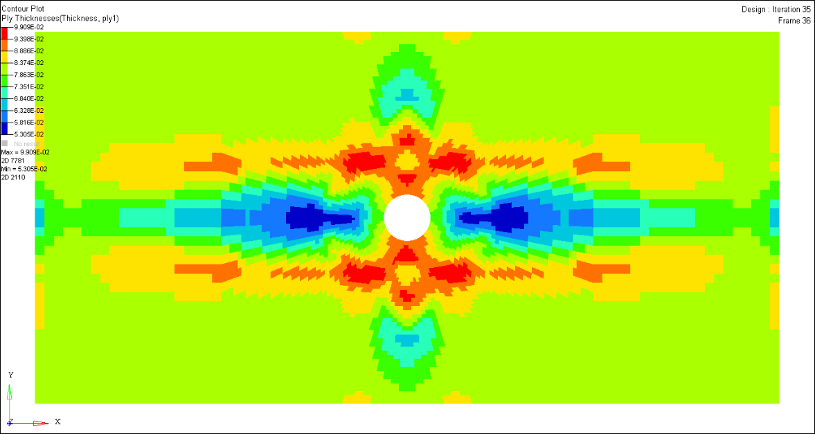
-
Contour panelでLayers 2、3および4を選択することにより、それぞれスーパープライ2(45°)、3(-45°)、および4(90°)のプライ板厚コンターを作成します。
適用されているバランス制約条件のために、+45°と-45°のスーパープライの板厚分布は同じです。
図 11. -45/+45度のスーパープライのプライ板厚コンタープロット 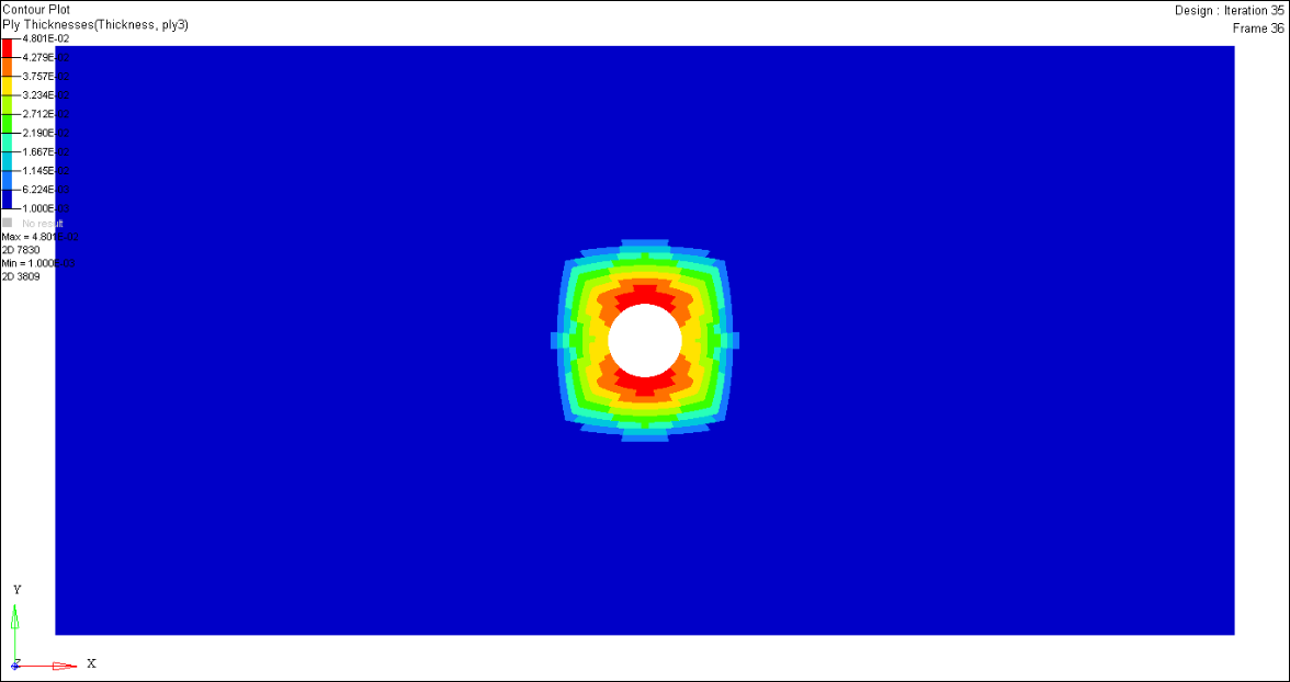
図 12. 90度のスーパープライのプライ板厚コンタープロット 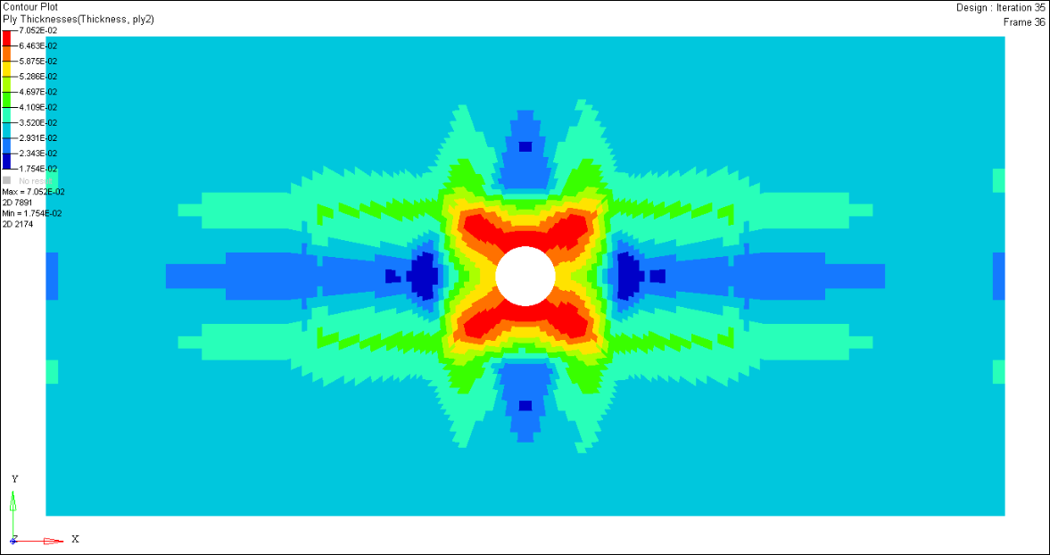
プライバンドルの表示
- HyperMeshに戻り、新しいモデルを開始します。
- ファイルoht_opti_ph1.femと同じディレクトリにあるソルバーデックoht_opti_ph1_sizing.*.incを、現在のセッションにインポートします。
-
Model Browserで、Load
Collectors欄を右クリックし、context menuからHideを選択します。
すべての荷重コレクターの表示がオフになります。
-
Model Browserで、Plies欄を右クリックし、コンテキストメニューからHideを選択します。
すべてのプライの表示がオフになります。
-
Model BrowserのPliesフォルダーで、それぞれ各プライについてメッシュビューアイコンをアクティブにし、プライを確認します。
図 13. プライ11300が選択されているModel Browserビュー(Laminate 1, Ply 1, Shape 3) 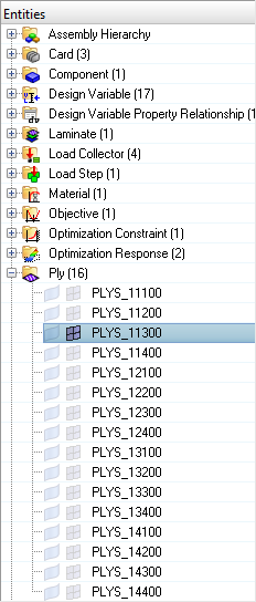
図 14. プライ11300のグラフィックス領域のビュー(Laminate 1, Ply 1, Shape 3) 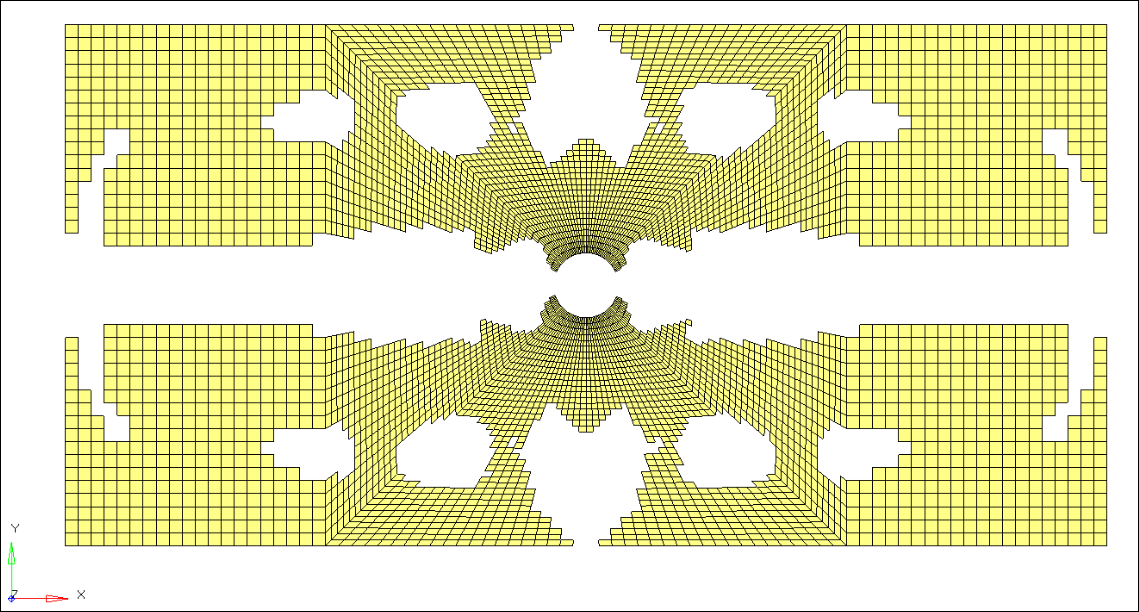
OSSmoothを使ったプライスムージングの適用
- PostページからOSSmoothパネルをクリックします。
- Select model欄で、oht_opti_ph1_sizing.35.femを選択します。
- modeをGeometryからPLY Shapeに変更します。
- output file欄で、oht_opti_ph1_sizing.35.smoothed.femの名称を擁す元の場所にセットします。
- smooth iterations欄に20と入力します。
- small regionの下で、split disconnectedとcreate geometryのボックスからチェックマークを外します。
- area ratio欄に0.010と入力します。
- OSSmoothをクリックし、解析を実行してモデルをスムージングします。