
OS-T:4070 飛行機の翼のリブの非線形ギャップを用いたフリー寸法最適化
本チュートリアルではアルミニウム製の翼小骨(リブ)をモデル化した既存の有限要素モデルを使用し、フリー寸法最適化を行う方法について説明します。
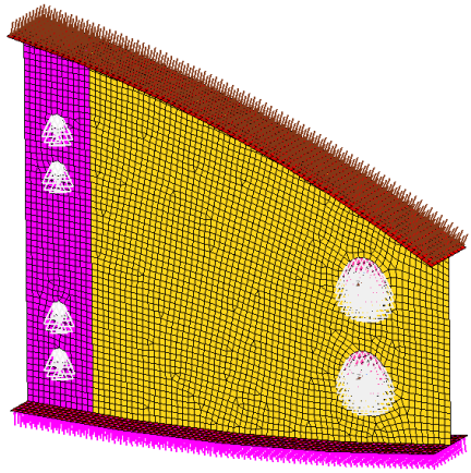
モデル内には、取り付けフランジ、ウェブ(薄い金属板)、上部と下部のフランジおよびラグ(肉厚を部分的に厚くした突起部)の4つのシェルコンポーネントがあります。ウェブはギャップ要素でラグと結合しています。適切な材料特性、荷重、境界条件および非線形サブケースが既にモデルに定義されています。設計領域はウェブで、残りのコンポーネントは非設計領域です。航空宇宙関連の部品の大部分は機械加工またはフライス加工で製造されたシェル構造で、フリー寸法最適化はこれらの部品に非常に適しています。トポロジー最適化適用の限界を理解するために、非線形ギャップを用いたトポロジー最適化を翼のリブモデルで実施します。
- 目標
- 重み付きコンプライアンスWCOMPの最小化
- 制約条件
- ウェブの体積率 < 0.3
- フリー寸法最適化の設計変数:
- 設計領域での各シェル要素の板厚
- トポロジー最適化の設計変数
- 設計領域での各シェル要素の要素密度
HyperMeshの起動とOptiStructユーザープロファイルの設定
使用されるモデルは、図 6に示すようなコントロールアームのモデルです。荷重と拘束条件、および2つの静的荷重ケースは、このモデルに既に定義されています。
本演習に使用されるモデルは、OS-T:6030 シーム溶接疲労解析、S-N法OS-T:6040 S-N法を用いたスポット溶接疲労解析図 1に示すような自動車のフレームのモデルです。入力ファイルには、フレームが受ける3つの静的荷重ステップFrontal torsion、Rear torsionおよびVertical bendingです。
本演習に使用されるモデルは、図 1に示すようなシンプルなCADボックスのモデルです。4つの荷重ステップは既にこのモデル上で定義されており、それぞれNormal Modes Analysis(ノーマルモード解析)、両方の拘束ポイントにおけるFrequency Response(周波数応答)およびRandom Response Analysis(ランダム応答解析)を表します。
本演習に使用されるモデルは、図 1に示すようなbracket_frf_ENのモデルです。3つの荷重ステップは既にこのモデル上で定義されており、それぞれStatic Analysis(静解析)、Normal Modes Analysis(ノーマルモード解析)および荷重位置において加振されるFrequency Response(周波数応答)。
-
HyperMeshを起動します。
User Profilesダイアログが現れます。
-
OptiStructを選択し、OKをクリックします。
これで、ユーザープロファイルが読み込まれます。ユーザープロファイルには、適切なテンプレート、マクロメニュー、インポートリーダーが含まれており、OptiStructモデルの生成に関連したもののみにHyperMeshの機能を絞っています。
- をクリックします。
- New Sessionで、作業ディレクトリフォルダーに名称を入力します。
-
Createをクリックします。
これで、現在ロードされている疲労プロセステンプレートの内容を保存するための新しいファイルが生成されます。
フリー寸法非線形ギャップ最適化の実行
モデルのオープン
- をクリックします。
- 自身の作業ディレクトリに保存したrib_complete.hmファイルを選択します。
-
Openをクリックします。
rib_complete.hmデータベースが現在のHyperMeshセッションに読み込まれます。
最適化のセットアップ
フリー寸法最適化設計変数の作成
- Analysisページからパネルoptimizationをクリックします。
- free sizeパネルをクリックします。
- createサブパネルを選択します。
- desvar=欄にshellsと入力します。
- typeをPSHELLにセットします。
- プロパティセレクターを使って、Webコンポーネントを選択します。
- createをクリックします。
フリー寸法製造用制約条件の作成
- parametersサブパネルを選択します。
- desvarsをクリックしshellsを選択します。
- minmemb offからmindim =に切り替え、2.0と入力します。
- updateをクリックします。
- returnをクリックします。
Create Optimization Responses
- From the Analysis page, click optimization.
- Click Responses.
-
Create the volume fraction response.
- In the responses= field, enter Volfrac.
- Below response type, select volumefrac.
- Set regional selection to total and no regionid.
- Click create.
-
Create the weighted component response.
- In the responses= field, enter wcomp.
- Below response type, select weighted comp.
- Click loadsteps, then select all loadsteps.
- Click return.
- Click create.
- Click return to go back to the Optimization panel.
Create Design Constraints
- Click the dconstraints panel.
- In the constraint= field, enter vol.
- Click response = and select volfrac.
- Check the box next to upper bound, then enter 0.3.
- Click create.
- Click return to go back to the Optimization panel.
Define the Objective Function
- Click the objective panel.
- Verify that min is selected.
- Click response= and select wcomp.
- Click create.
- Click return twice to exit the Optimization panel.
Run the Optimization
- From the Analysis page, click OptiStruct.
- Click save as.
-
In the Save As dialog, specify location to write the
OptiStruct model file and enter
rib_freesize for filename.
For OptiStruct input decks, .fem is the recommended extension.
-
Click Save.
The input file field displays the filename and location specified in the Save As dialog.
- Set the export options toggle to all.
- Set the run options toggle to optimization.
- Set the memory options toggle to memory default.
-
Click OptiStruct to run the optimization.
The following message appears in the window at the completion of the job:
OPTIMIZATION HAS CONVERGED.
FEASIBLE DESIGN (ALL CONSTRAINTS SATISFIED).
OptiStruct also reports error messages if any exist. The file rib_freesize.out can be opened in a text editor to find details regarding any errors. This file is written to the same directory as the .fem file. - Click Close.
- rib_freesize.hgdata
- HyperGraph file containing data for the objective function, percent constraint violations, and constraint for each iteration.
- rib_freesize.hist
- The OptiStruct iteration history file containing the iteration history of the objective function and of the most violated constraint. Can be used for a xy plot of the iteration history.
- rib_freesize.HM.comp.tcl
- HyperMesh command file used to organize elements into components based on their density result values. This file is only used with OptiStruct topology optimization runs.
- rib_freesize.HM.ent.tcl
- HyperMesh command file used to organize elements into entity sets based on their density result values. This file is only used with OptiStruct topology optimization runs.
- rib_freesize.html
- HTML report of the optimization, giving a summary of the problem formulation and the results from the final iteration.
- rib_freesize.mvw
- HyperView session file.
- rib_freesize.oss
- OSSmooth file with a default density threshold of 0.3. You may edit the parameters in the file to obtain the desired results.
- rib_freesize.out
- OptiStruct output file containing specific information on the file setup, the setup of the optimization problem, estimates for the amount of RAM and disk space required for the run, information for all optimization iterations, and compute time information. Review this file for warnings and errors that are flagged from processing the rib_freesize.fem file.
- rib_freesize.res
- HyperMesh binary results file.
- rib_freesize.sh
- Shape file for the final iteration. It contains the material density, void size parameters and void orientation angle for each element in the analysis. This file may be used to restart a run.
- rib_freesize.stat
- Contains information about the CPU time used for the complete run and also the break-up of the CPU time for reading the input deck, assembly, analysis, convergence, and so on.
- rib_freesize_des.h3d
- HyperView binary results file that contain optimization results.
- rib_freesize_frame.html
- HTML file used to post-process the .h3d with HyperView Player using a browser. It is linked with the _menu.html file.
- rib_freesize_hist.mvw
- Contains the iteration history of the objective, constraints, and the design variables. It can be used to plot curves in HyperGraph, HyperView, and MotionView.
- rib_freesize_menu.html
- HTML file used to post-process the .h3d with HyperView Player using a browser.
- rib_freesize_s#.h3d
- HyperView binary results file that contains from linear static analysis, and so on.
- rib_freesize.fsthick
- The element definitions for those elements that were part of a free size design space. The optimized thickness of these elements is provided as nodal thickness values (Ti).
結果の表示
-
OptiStructパネルから、HyperViewをクリックします。
HyperViewがHyperMesh Desktop内で起動し、rib_freesize.h3dファイルからの結果が読み込まれます。
-
Visualizationツールバーで
 をクリックし、Entity Attributesパネルを開きます。
-
Auto appy mode: Display Offを選択し、Webコンポーネントを選択します。
Web以外のコンポーネントはすべて表示されていません。
-
Mesh影付メッシュオプション
 をクリックします。
- Webコンポーネントをクリックし、影付きのメッシュにします。
-
Resultsツールバーで
 をクリックし、Contour panelを開きます。
- Result typeをElement Thicknessesに設定します。
-
Results Browserから、Simulationリストにリストされている最終反復計算を選択します。
図 2. 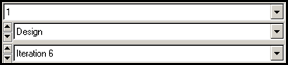
-
Standard Viewsツールバーで
 をクリックし、Webをトップビューで表示させます。
Webコンポーネントの要素板厚コンターが表示されます。
フリー寸法最適化の結果は、製造プロセスを簡略化するために大規模な範囲の中で板厚を削減することができるような最適化された板厚分布のウェブとなります。また、フリー寸法から得られた設計はトポロジー最適化では得ることのできない空洞、リブおよび連続的に変化する板厚を同時に生成する自由度を提供します。図 3. フリー寸法非線形ギャップ最適化による板厚コンター. プレート板厚0.1mmのWebの 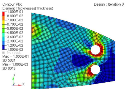
-
Page Controlsツールバーで
 をクリックし、HyperMeshクライアントが表示されるまで、HyperViewクライアントページを閉じます。
データベースの保存
- menu barでをクリックします。
- Save Asダイアログでファイル名欄にrib_complete.hmと入力し、自身の作業ディレクトリに保存します。
トポロジー非線形ギャップ最適化の実行
非線形ギャップ要素を用いたトポロジー最適化のセットアップ
トポロジー設計変数の作成
- Model Browserで、Design Variable欄を右クリックし、context menuからDeleteを選択します。
- Analysisページからパネルoptimizationをクリックします。
- topologyパネルをクリックします。
- createサブパネルを選択します。
- desvar=欄にshellsと入力します。
- プロパティセレクターを使って、Webコンポーネントを選択します。
- typeをPSHELLにセットします。
- base thicknessは0.0のままとします。
- createをクリックします。
データベースの保存
- menu barでをクリックします。
- Save Asダイアログでファイル名欄にrib_topology.hmと入力し、自身の作業ディレクトリに保存します。
トポロジー最適化製造用制約条件の作成
- parametersサブパネルを選択します。
- desvars =をクリックしshellsを選択します。
- minmemb offをmindim =に切り替え、最小部材寸法制御として2.0を入力します。
- updateをクリックします。
- returnを2回クリックします。
Run the Optimization
- From the Analysis page, click OptiStruct.
- Click save as.
-
In the Save As dialog, specify location to write the
OptiStruct model file and enter
rib_topology for filename.
For OptiStruct input decks, .fem is the recommended extension.
-
Click Save.
The input file field displays the filename and location specified in the Save As dialog.
- Set the export options toggle to all.
- Set the run options toggle to optimization.
- Set the memory options toggle to memory default.
-
Click OptiStruct to run the optimization.
The following message appears in the window at the completion of the job:
OPTIMIZATION HAS CONVERGED.
FEASIBLE DESIGN (ALL CONSTRAINTS SATISFIED).
OptiStruct also reports error messages if any exist. The file rib_topology.out can be opened in a text editor to find details regarding any errors. This file is written to the same directory as the .fem file. - Click Close.
結果の表示
-
OptiStructパネルから、HyperViewをクリックします。
HyperViewがHyperMesh Desktop内で起動し、rib_topology.mvwファイルからの結果が読み込まれます。このファイルは、モデルと結果が定義されている.h3dファイルとリンクされています。
-
Visualizationツールバーでをクリックし、Entity Attributesパネルを開きます。
-
Auto appy mode: Display Offを選択し、Webコンポーネントを選択します。
Web以外のコンポーネントはすべて表示されていません。
-
Mesh影付メッシュオプションをクリックします。
- Webコンポーネントをクリックし、影付きのメッシュにします。
-
Resultsツールバーでをクリックし、Contour panelを開きます。
- Result typeをElement Densitiesに設定します。
- Results Browserから、Simulationリストにリストされている最終反復計算を選択します。
-
Standard Viewsツールバーでをクリックし、Webをトップビューで表示させます。
- Applyをクリックし、Webコンポーネントの要素密度のコンターを表示させます。
フリー寸法最適化およびトポロジー最適化の結果の確認と比較
トポロジー最適化の結果は、材料を完全に残す部分と削除する部分(空洞)から成るトラスタイプの構造を示し、フリー寸法最適化の結果は、板厚が連続的に変化するようなせん断パネルタイプの構造を示す傾向があります。ソリッドモデルに関しては、要素を完全に残すか削除するか以外に選択の余地がありませんが、シェルモデルに関しては、トポロジー最適化のペナルティ係数(opti controlパネルのDISCRETE)によって中間的な密度をもつ要素が0か1どちらかの値に近くなるように変換されることで、必ずしも効率的とはいえない構造を導き出す場合もあります。また、航空宇宙関連の構造物の大半は板構造であり、切削加工などの製造条件によりせん断パネルタイプの構造物がしばしば必要とされます。フリー寸法最適化は、このような場合に非常に有効です。