The first step in defining the
loading sequence is to define the TABFAT curves. This represents
the loading history.
Make sure the Utility menu is selected in the View
menu. Click View > Browsers > HyperMesh > Utility.
Click on the Utility menu beside the Model tab in the
browser. In the Tools section, click on TABLE
Create.
Set Options to Import table.
Set Tables to TABFAT.
Click Next.
Browse for the loading file.
In the Open the XY Data File dialog box, set the Files of
type filter to CSV (*.csv).
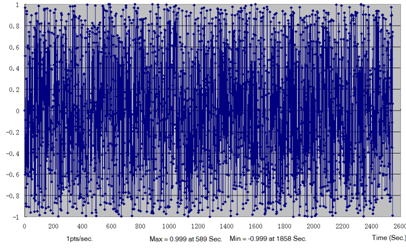
Open the load1.csv file you saved to your working directory.
Create New Table with Name table1.
Click Apply to save the table.
The curve table1 with
TABFAT card image is created.
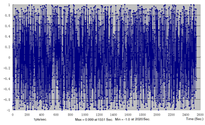
Browse for a second loading file load2.csv.
Create New Table with Name table2.
Click Apply to save the table.
The curvetable2 with TABFAT card image is
created.
Exit from the Import TABFAT window.
Tables appear under Curve in the Model Browser.
注: A file in DAC format can very
easily be imported in HyperGraph and converted
to CSV format to be read in HyperMesh.
Define FATLOAD Load Collector
In the Model Browser, right-click and select Create > Load Collector.
For Name, enter FATLOAD1.
Click Color and select a color from the color
palette.
For Card Image, select FATLOAD.
For TID(table ID), select table1 from the list
of curves.
For LCID (load case ID), select SUBCASE1 from the
list of load steps.
Set LDM (load magnitude) to 1.
Set Scale to 3.0.
Repeat the process to create another load collector named
FATLOAD2 with FATLOAD Card
Image and pointing to table2 and
SUBCASE2.
Set LDM to 1 and Scale to 3.0.
Define FATEVNT Load Collector
In the Model Browser, right-click and select Create > Load Collector.
For Name, enter FATEVENT.
For Card Image, select FATEVNT.
For FATEVNT_NUM_FLOAD, enter 2.
Click on the Table icon
next to the Data field and select FATLOAD1 for FLOAD(1)
and FATLOAD2 for FLOAD(2) in the pop-out window.
Define FATSEQ Load Collector
In the Model Browser, right-click and select Create > Load Collector.
For Name, enter FATSEQ.
For Card Image, select FATSEQ.
For FID (Fatigue Event Definition), select FATEVENT
.
Defining the sequence of events for the fatigue analysis is completed.
The Fatigue parameters are defined next.
Define Fatigue Parameters
In the Model Browser, right-click and select Create > Load Collector.
For Name, enter fatparam.
For Card Image, select FATPARM.
Verify TYPE is set to SN.
Set MAXLFAT to Yes for the
multiaxial method.
Set STRESSU to MPA (Stress Units).
Set RAINFLOW RTYPE to LOAD.
Define Fatigue Material Properties
The material curve for the fatigue analysis can be defined on the
MAT1 card.
In the Model Browser, click on the MAT1 material.
The Entity Editor opens.
In the Entity Editor, set MATFAT to SN.
Set UTS (ultimate tensile stress) to 600.
For the SN curve set (these values should be
obtained from the material's SN curve):
SRI1
1903.0
B1
-0.123
NC1
1e6
B2
0.0
FL
0.0
SE
0.0
Define PFAT Load Collector
In the Model Browser, right-click and select Create > Load Collector.
For Name, enter pfat.
For Card Image, select PFAT.
Set LAYER to TOP.
Set FINISH to NONE.
Set TRTMENT to NONE.
Set Kf to 1.0.
Define FATDEF Load Collector
In the Model Browser, right-click and select Create > Load Collector.
For Name, enter fatdef.
Set the Card Image to FATDEF.
Select the PTYPE check box and activate
PSOLID.
Edit FATDEF_PSOLID_NUMIDS to 2. The model contains 2 solid properties defined in the model.
Click on the Table icon
next to the Data field and select PSOLID_2 for PID(1),
pfat for PFATID(1) and
PSOLID_5 for PID(2) and pfat
for PFATID(1) in the pop-out window.
Click Close.
Define the Fatigue Load Step
In the Model Browser, right-click and select Create > Load Step.

 を選択します。
Select OptiStruct Fileブラウザが開きます。
を選択します。
Select OptiStruct Fileブラウザが開きます。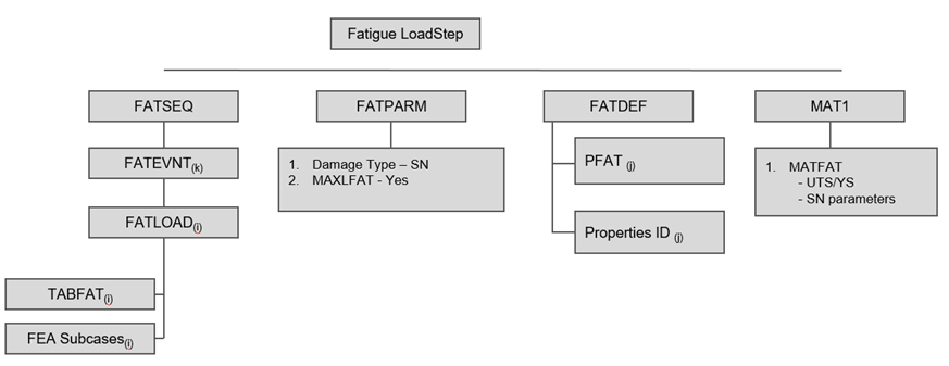
 next to the Data field and select FATLOAD1 for FLOAD(1)
and FATLOAD2 for FLOAD(2) in the pop-out window.
next to the Data field and select FATLOAD1 for FLOAD(1)
and FATLOAD2 for FLOAD(2) in the pop-out window.
 をクリックし、Contour panelを開きます。