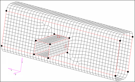
In this tutorial you will perform a shape optimization on a rail-joint. The
rail-joint is made of shell elements and has one load case. The shape of the joint is
modified to satisfy stress constraints while minimizing mass.
Before you begin, copy the file(s) used in this tutorial to your
working directory.
Shape optimization requires you to have knowledge of the kind of shape you would like
to change in the structure. This may include finding the optimum shape to reduce
stress concentrations to changing the cross-sections to meet specific design
requirements. Therefore, you need to define the shape modifications and the nodal
movements to reflect the shape changes. Shape optimization requires the use of two
cards DESVAR and DVGRID. They can be defined
using HyperMorph. Then these cards are included in the
OptiStruct input file along with the objective
function and constraints to run the shape optimization.Figure 1. Rail Joint
The optimization problem for this tutorial is stated as:
Objective
Minimize mass.
Constraints
Maximum von Mises stress of the joint < 200 MPa.
Design Variables
Shape variables.
Launch HyperMesh and Set the OptiStruct User Profile
Launch HyperMesh.
The User Profile dialog opens.
Select OptiStruct and click
OK.
This loads the user profile. It includes the appropriate template, macro
menu, and import reader, paring down the functionality of HyperMesh to what is relevant for generating models for
OptiStruct.
Open the Model
Click File > Open > Model.
Select the rail_joint_original.hm file you saved to
your working directory.
Click Open.
The rail_joint_original.hm database is loaded
into the current HyperMesh session, replacing any
existing data.
Submit the Job
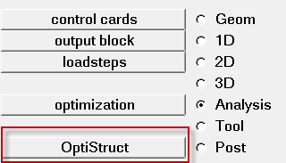
From the Analysis page, click the OptiStruct
panel.
Figure 2. Accessing the OptiStruct Panel
Click save as.
In the Save As dialog, specify location to write the
OptiStruct model file and enter
rail_joint_original for filename.
For OptiStruct input decks,
.fem is the recommended extension.
Click Save.
The input file field displays the filename and location specified in the
Save As dialog.
Set the export options toggle to all.
Set the run options toggle to analysis.
Set the memory options toggle to memory default.
Click OptiStruct to launch
the OptiStruct job.
If the job is successful, new results files
should be in the directory where the rail_joint_original.fem was written. The rail_joint_original.out file is a good place to look for error messages that could help
debug the input deck if any errors are present.
View the Results
HyperView is a complete post-processing and visualization
environment for finite element analysis (FEA), multibody system simulation, video and
engineering data.
From the OptiStruct panel, click HyperView.
HyperView launches within the HyperMesh Desktop and loads the result
file(s).
On the Results toolbar, click to
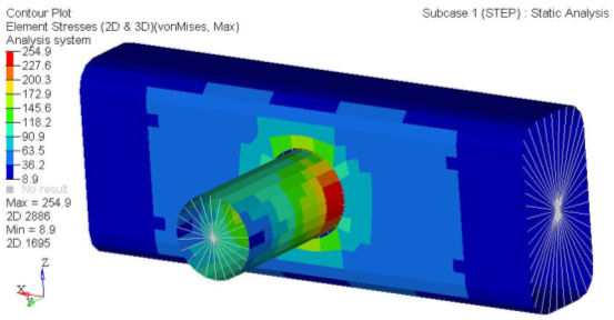
open the Contour panel.
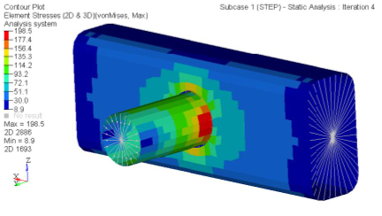
Set the Result type to Element Stresses [2D & 3D]
(t) and von Mises.
Click Apply.
Take note of the Maximum von Mises Stress of the joint.Figure 3. von Mises Stress for the Intial Design
From the Page Controls toolbar, click to
delete the page within the HyperView client.
You should now be on Page 1 in the HyperMesh
client.
Click return to exit the panel.
Set Up the Model
Display Node IDs
From the Tool page, click the numbers panel.
Click nodesby sets.
Select node set.
Click select.
Sixteen (16) nodes are highlighted.
Click on to display node IDs.
Click return.
Build 2D Domains on the Rail
In the Model Browser, Component folder, right-click on
PSHELL and select Isolate from
the context menu.
All components except PSHELL are turned off for ease
of visualization.
From the Analysis page, click the optimization
panel.
Click the HyperMorph panel.
Click the domains panel.
Edit partitioning settings.
Select the partitioning subpanel.
For domain angle =, enter 50.
For curve tolerance =, enter 8.0000.
Create domains.
Select the create subpanel.
Switch from global domains to 2D domains.
Switch all elements to elems.
Click elems > by sets.
Select rail_set1 and
rail_set2, then click
select.
Click create.
Figure 4. Rail Domains
Split the Circular Edge Domains Around the Opening of the Rail
In this step you will split each of the two circular domains into four curved edge
domains.
Select edit edges subpanel.
Set the top selector to split.
Split the first circular edge-domain.
Using the domain selector, select the circular edge-domain passing
through nodes 1300, 1305, 1311, and 1316.
Using the node selector, select node 1311.
Click split.
The circular domain is split at node 1311 and a new handle is
created at node 1311.
Using the domains selector, select the circular edge between node 1311
and the other handle.
Using the node selector, select node 1316.
Click split.
Split the curved edge at nodes 1305 and 1300, respectively.
Split the circular domain using the four nodes on the other side of the
rail.
Using the domain selector, select the circular edge-domain passing
through nodes 931, 926, 937 and 942.
Using the node selector, select node 931.
Click split.
Using the domain selector, select the circular edge between node 931
and the other handle.
Using the node selector, select node 926.
Click split.
Split the curved edge at nodes 937 and 942, respectively.
Figure 5. Rail Domains After The Circular Edge Have Been Split
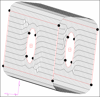
Merge Edge Domains
Each circular domain on the rail has been split at four nodes and four new handles have
been added to each circular domain. This operation results in five curved edge domains
on each circular edge on the rail. The objective is to have only four domains. In this
step you will merge domains.
In the edit edges subpanel, switch from split to
merge.
Merge the domains between nodes 926 and 924.
Using the domain selector, select the outer red curve from node 926 to
pre-existing handle.
Select the outer red curve from pre-existing handle to node 942.
Uncheck retain handles.
Click merge.
The pre-existing handle is removed.
Merge the domains between nodes 1316 and 1300.
Figure 6. Rail Domains After Few Domains Are Merged
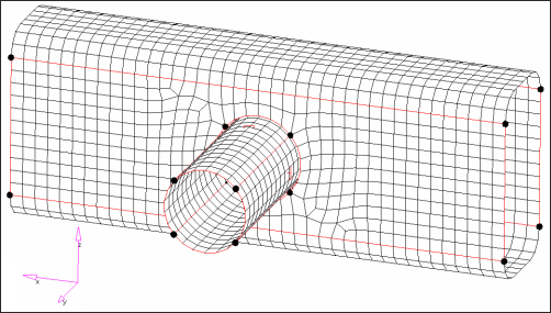
Build 2D Domains on the Tube
In the Model Browser, Component folder, right-click on
PSHELL.1 and select Show from
the context menu.
In the domains panel, select the create subpanel.
Set the top selector to 2D domains.
Create a domain for the element set, elem_set1.
Click elems > by sets.
Select elem_set1, then click
select.
Click create.
Create three more 2D domains for elements in sets elem_set2, elem_set3, and
elem_set4.
Click return and go back to the HyperMorph module.
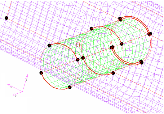
Figure 7. Domains on Rail and Tube Joint
Create Shapes
In this step you will create shapes using the created domains and handles.
Click the morph panel.
Modify the curvatures of selected edge domains for the first shape.
Select the alter dimensions subpanel.
The alter dimensions subpanel can be used to modify the curvatures of
selected edge domains.
Set the first switch to curve ratio.
Set center calculation to by edges.
Under the edges only: domains selector, set the switch to
hold ends.
Holding two ends of a selected edge domain allows a change of
curvature of the selected edge without altering its end points.
Leave the other settings with the defaults.
Using the domains selector, select the red edge-domains.
Tip: You might need to zoom in for easier picking
operation.
A total of eight edge domains are selected and highlighted.Figure 8. Morph edge Domains
In the curve ratio = and enter 20.
Click morph.
A new curvature is applied to the selected eight edge
domains.
Save the shape, sh1.
Select the save shape subpanel.
In the shape= field, enter sh1.
Toggle as handle perturbation to as node
perturbation.
Click color and change the color of the shape
vectors or leave the default color.
Click save.
Shape vectors (arrows) are created of the selected color.Figure 9. Shape Variable, sh1.
Click undo all to prepare for the generation of the next
shape.
In the Model Browser, right-click on
Shape and select Hide from the
context menu.
Select the alter dimensions subpanel.
Next to the domains selector, click to
reset and remove any previous selections.
Modify the curvatures of selected edge domains for the first shape.
Using the domains selector, select the red edge curves.
Figure 10. Morph Edge Domains For The Second Shape
Click morph.
A new curvature is applied to the selected eight edge
domains.
Save the shape, sh2.
Select the save shape subpanel.
In the shape= field, enter sh2.
Toggle as handle perturbation to as node
perturbation.
Click color and change the color of the shape
vectors or leave the default color.
Click save.
Figure 11. Shape Variable, sh2
Click undo all to prepare for the generation of the next
shape.
In the Model Browser, right-click on
Shape and select Hide from the
context menu.
Create a new shape as a linear combination of existing shapes.
Select the apply shapes subpanel.
Using the shapes selector, select sh1 and
sh2.
In the multiplier= field, enter 1.0.
Click apply.
Save the shape, sh3.
Select the save shape subpanel.
In the shape= field, enter sh3.
Toggle as node perturbation to as handle
perturbation.
Click color and change the color of the shape
vectors or leave the default color.
Click save.
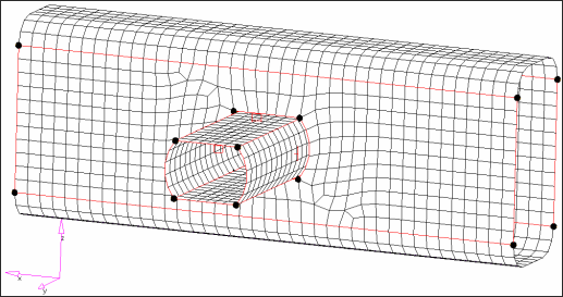
The new shape, sh3, includes influences from both sh1 and sh2
shapes.Figure 12. Shape Variable, sh3. This shape variable converts the tube to a square
cross-section.
CAUTION: Do not click undo all at this moment,
because one more shape based on this third shape change will be created.
In the Model Browser, right-click on
Shape and select Hide from the
context menu.
In the Model Browser, Component folder, right-click
PSHELL and click Hide from the
context menu.
The component is turned off for ease of visualization.
Modify the curvatures of selected edge domains for the first shape.
Select the alter dimensions subpanel.
Next to the domains selector, click to reset and remove any previous selections.
Switch the top selector from curve ratio to
distance.
This feature allows you to shorten the distance between selected
domains.
Set end a to nodes and handles.
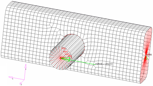
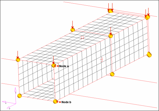
Using the node a and node b selectors, select the nodes indicated in
Figure 13.
Figure 13.
Once nodes a and b are selected, the distance between node a and
node b is measured automatically and appears in distance = field. The
distance between node a and node b is about 43.
Under followers (end a), use the handles selector to select the eight
handles shown by the downward pointing arrows in Figure 13.
Under followers (end b), use the handles selector to select the eight
handles near the opposite face of the tube.
Set the bottom selector to hold middle.
These components are turned on for ease of visualization.
In the distance= field, enter 20.
Click morph.
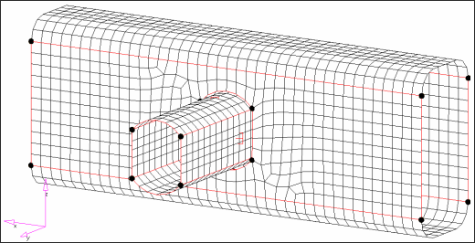
A rectangular shape appears to the joint.
Save the shape, sh4.
Select the save shape subpanel.
In the shape= field, enter sh4.
Toggle as handle perturbation to as node
perturbation.
Click color and change the color of the shape
vectors or leave the default color.
Click save.
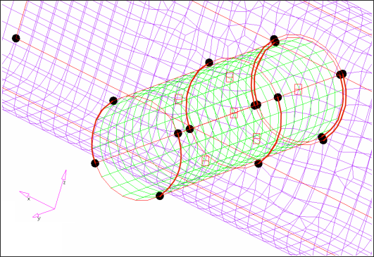
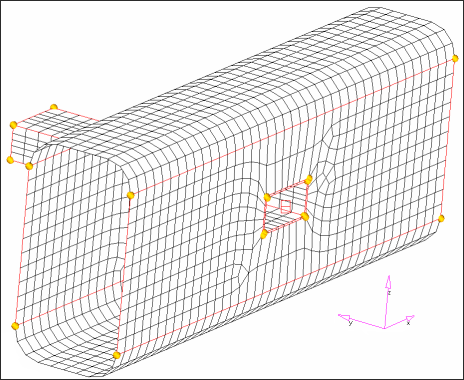
Figure 14. Shape Variable, sh4
Click undo all to restore the mesh to the baseline
configuration.
In the Model Browser, right-click on
Shape and select Hide from the
context menu.
Click return three times to go the main menu.
Set Up the Optimization
Define the Shape Design Variables and Review Animation
From the Analysis page, click the optimization
panel.
Click the shape panel.
Select the desvar and create
subpanels.
Set single desvar to multiple desvars.
Create shape design variables.
Using the shapes selector, select sh1,
sh2, sh3 and
sh4.
In the initial value = field, enter 0.0.
In the lower bound = field, enter -1.0.
In the upper bound = field, enter 1.0.
Click create.
Four design variables are created with the same initial value, lower
bound, and upper bound. HyperMesh automatically
links the design variables to each shape, respectively and assigns names to each
design variable the same as its associated shapes.
Animate the shapes.
Click animate.
Click simulation= and select
SHAPE-sh1(1).
Set data type= to Perturbation vector.
Click modal.
Click next and then
animate to see the next shape variable, and
so forth.
Click return three times to go back to the Optimization panel.
Create Optimization Responses
From the Analysis page, click optimization.
Click Responses.
Create the mass response, which is defined for the total volume of the
model.
In the responses= field, enter mass.
Below response type, select mass.
Set regional selection to total and
no regionid.
Click create.
Create a static stress response.
In the response= field, enter Stress.
Set the response type to static stress.
Using the props selector, select PSHELL.1.
Set the response selector to von mises.
Under von mises, select both surfaces.
Click create.
Click return to go back to the Optimization panel.
Define the Objective Function
Click the objective panel.
Verify that min is selected.
Click response and select Mass.
Click create.
Click return twice to exit the Optimization panel.
Create Design Constraints
Click the dconstraints panel.
In the constraint= field, enter con.
Click response = and select Stress.
Check the box next to upper bound, then enter
200.
Using the loadsteps selector, select STEP.
Click create.
Click return to go back to the Optimization panel.
Define Control Cards for Shape Optimization
Without this control card defined, optimization gets terminated by quality check and you do
not get the converged results.
From the Analysis page, click the control cards
panel.
In the Card Image dialog, click PARAM.
Select CHECKEL.
Set CHECKEL_V1 to NO.
Click return twice.
Run the Optimization
From the Analysis page, click OptiStruct.
Click save as.
In the Save As dialog, specify location to write the
OptiStruct model file and enter
rail_joint_opt for filename.
For OptiStruct input decks,
.fem is the recommended extension.
Click Save.
The input file field displays the filename and location specified in the
Save As dialog.
Set the export options toggle to all.
Set the run options toggle to optimization.
Set the memory options toggle to memory default.
Click OptiStruct to run the optimization.
The following message appears in the window at the completion of the
job:
OPTIMIZATION HAS CONVERGED.
FEASIBLE DESIGN (ALL CONSTRAINTS SATISFIED).
OptiStruct also reports error messages if any exist. The
file rail_joint_opt.out can be opened in a
text editor to find details regarding any errors. This file is written to the
same directory as the .fem file.
Click Close.
View the Results
Review the Shape Optimization Results
From the OptiStruct panel, click HyperView.
HyperView is launched and the results are
loaded. A message window appears to inform of the successful model and result
files loading into HyperView.
On the Results toolbar, click to open the
Contour panel.
Set the Result type to Shape Change [v] and
mag.
Shape Change [v] should be the only results type in the rail_joint_opt_des.h3d file.
Click Apply.
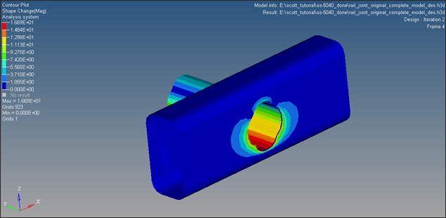
The shape change displays. The contour is all blue because your results
are on the first design step or Iteration 0.
In the Results Browser, select the last iteration.
Each element of the model is assigned a legend color, indicating the
density of each element for the selected iteration. Shape optimization results
are applied to the model.Figure 15. Figure 16. Shape Change Converged (Scale 2x)
View a Contour Plot of the Stress
In the top, right of the application, click to proceed to page 2.
On the Results toolbar, click to open the
Contour panel.
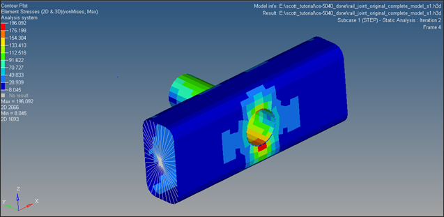
Set the Result type to Element Stresses [2D & 3D]
[t] and von Mises.
In the Results Browser, select the last iteration.
Click Apply.
The stress
contour shows on top of the shape changes applied to the model. Verify that this value
is around the constraint value specified.Figure 17. von Mises Stress for the Last Iteration (Max < 200 MPa)
Review the Results
Is your design objective of minimizing the volume obtained? If not, can you explain
why?
Are your design constraints satisfied?
Which shape has the most influence in this problem setup?

 to
open the Contour panel.
to
open the Contour panel.
 to
delete the page within the HyperView client.
You should now be on Page 1 in the HyperMesh client.
to
delete the page within the HyperView client.
You should now be on Page 1 in the HyperMesh client.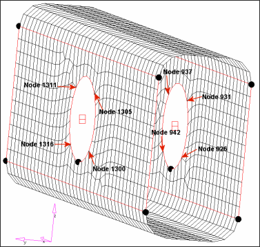

 to
reset and remove any previous selections.
to
reset and remove any previous selections.
 to open the
Contour panel.
to open the
Contour panel.

 to proceed to page 2.