OS-T: 2060 Symmetry and Draw Direction Constraints Applied
Simultaneously
In this tutorial you will perform a topology optimization on an automotive control
arm with the simultaneous application of symmetry and draw direction
constraints.
Before you begin, copy the file(s) used in this tutorial to your
working directory.
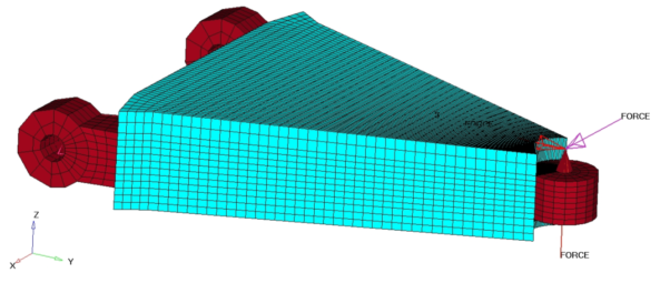
This tutorial uses the same optimization problem considered in OS-T: 2010 Design Concept for an Automotive Control Arm, except that a
refined mesh will be used in order to better capture the effect of applying
symmetric and draw manufacturing constraints simultaneously. The finite element mesh
of the structural model containing the designable (blue) and the non-designable
(red) regions, along with the loads and constraints applied.Figure 1.
The optimization problem is stated as:
Objective
Minimize volume.
Constraints
SUBCASE 1: The resultant displacement of the point where loading is
applied must be less than 0.05 mm.
SUBCASE 2: The resultant displacement of the point where loading is
applied must be less than 0.02 mm.
SUBCASE 3: The resultant displacement of the point where loading is
applied must be less than 0.04 mm.
Design Variables
Element density.
Launch HyperMesh and Set the OptiStruct User Profile
Launch HyperMesh.
The User Profile dialog opens.
Select OptiStruct and click
OK.
This loads the user profile. It includes the appropriate template, macro
menu, and import reader, paring down the functionality of HyperMesh to what is relevant for generating models for
OptiStruct.
Import the Model
Click File > Import > Solver Deck.
An Import tab is added to your tab menu.
For the File type, select OptiStruct.
Select the Files icon .
A Select OptiStruct file browser
opens.
Select the carm_draw_symm.fem file you saved
to your working directory.
Click Open.
Click Import, then click Close to
close the Import tab.
Set Up the Optimization
Define the Symmetry and Draw Direction Manufacturing Constraints
From Analysis page, click the optimization panel.
Click the topology panel.
Defining minimum member size.
Click review and select
solid.
Select the parameters subpanel.
Toggle minmemb off to mindim, and enter
16.0.
This forces the diameter or thickness of any structural member to be
higher than 16 mm; if this is not user-defined, OptiStruct automatically selects a minimum member
size based on the average mesh size (if a manufacturing constraint is
selected).Figure 2.
Click update to confirm the minimum member size
set up.
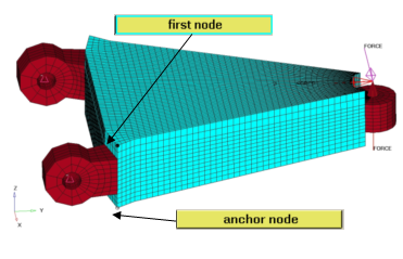
Defining the draw direction.
Select the draw subpanel.
Set draw type to single.
Using the anchor node and first node selectors, select the nodes
indicated in Figure 3.
Together, these two nodes define a vector in the positive Z direction.
This defines that the die draw direction is along the positive Z
direction.Figure 3.
Using the obstacle: props selector, select the
nondesign property.
Define the symmetry constraint.
Select the pattern grouping subpanel.
Set the pattern type to 1-pln sym.
Click anchor node, and enter
1 in the id= field.
The node with the ID of 1 is selected.
Click first node, and enter
2 in the id= field.
The node with the ID of 2 is selected.
Click update.
Together, these two nodes define a vector in the negative Z
direction. Hence, the symmetry plane is defined as the plane
perpendicular to the Z-axis (which is the same as the Y-Z plane), and
passing through the anchor node.
Click return twice to go back to the Analysis
page.
Run the Optimization
From the Analysis page, click OptiStruct.
Click save as.
In the Save As dialog, specify location to write the
OptiStruct model file and enter
carm_draw_symm_complete for filename.
For OptiStruct input decks,
.fem is the recommended extension.
Click Save.
The input file field displays the filename and location specified in the
Save As dialog.
Set the export options toggle to all.
Set the run options toggle to optimization.
Toggle memory options to upper limit in Mb and enter
2000.
Click OptiStruct to run the optimization.
The following message appears in the window at the completion of the
job:
OPTIMIZATION HAS CONVERGED.
FEASIBLE DESIGN (ALL CONSTRAINTS SATISFIED).
OptiStruct also reports error messages if any exist. The
file carm_draw_symm_complete.out can be opened in a
text editor to find details regarding any errors. This file is written to the
same directory as the .fem file.
Click Close.
View the Results
Element density results are output
to the carm_draw_symm_complete_des.h3d file from
OptiStruct for all iterations. In
addition, Displacement and Stress results are output for each subcase for
the first and last iterations by default into carm_draw_symm_complete_s#.h3d files, where # specifies
the sub case ID.
Review the Contour Plot of the Density Results
It is helpful to view the deformed shape of a model to determine if the boundary conditions
are defined correctly, and also to find out if the model is deforming as
expected. The analysis results are available in pages 2, 3, and 4. The
optimization iteration results (Element Densities) are loaded in the first
page.
From the OptiStruct panel, click
HyperView.
HyperView launches inside of
HyperMesh Desktop, and
all three .h3d files are loaded in a
different page.
In the top, right of the application, click to return to the Design History page, indicating that the
results correspond to optimization iterations.
From the Results toolbar, click to open the Contour panel.
Verify that the Result type is set to Element
Densities[s] and
Density.
This should be the only result type in the carm_draw_symm_complete_des.h3d
file.
Set the Averaging method to
Simple.
Click Apply to display the density
contour.
The contour is all blue because the results are on the
first design step or Iteration 0.
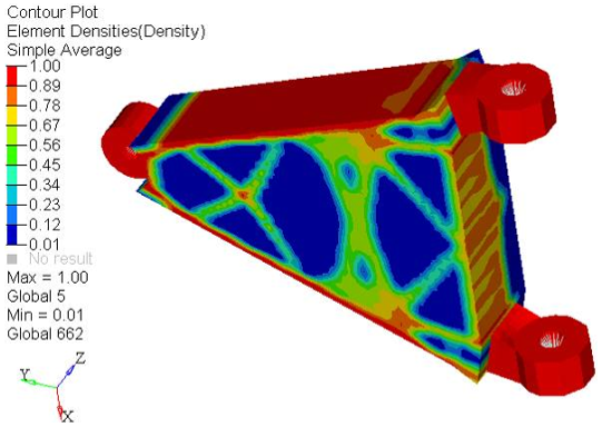
In the Results Browser, select the last
iteration listed.
Each element of the model is assigned a legend color,
indicating the density of each element for the selected
iteration.Figure 4.
View an Iso Value Plot of Element Densities
An Iso Value plot provides the information about the element density. Iso Value retains all
of the elements at and above a certain density threshold. Pick the density threshold
providing the structure that suits your needs.
From the Results toolbar, click to open the Iso Value panel.
Set the Result type to Element Densities.
Click Apply.
An Iso Plot displays.
Change the density threshold.
In the Current value field, enter 0.2.
Under Current value, move the slider.
When you update the density threshold, the Iso value displayed in the modeling window updates interactively. Use this tool to get a
better look at the material layout and the load paths from OptiStruct.
The parts of the model with densities greater than the specified value
of 0.2 display.Figure 5. Iso Value Plot of Element Densities
Review questions:
Have most of your elements converged to a density close to 1 or 0?
If there are many elements with intermediate densities, the
DISCRETE parameter may need to be adjusted. The
DISCRETE parameter (set in the opti control panel on
the Optimization panel) can be used to push elements
with intermediate densities toward 1 or 0, so that a more discrete structure
is given.
In this model, refining the mesh should provide a more discrete solution;
however, for the purposes of this tutorial, the current mesh and results are
sufficient.
Regions that need reinforcement tend towards a density of 1.0. Areas that do
not need reinforcement tend towards a density of 0.0.
Is the max= field showing 1.0e+00?
In this case, it is.
If it is not, the optimization has not progressed far enough. Allow more
iterations and/or decrease the OBJTOL parameter (also set
in the opti control panel).
If adjusting the discrete parameter, refining the mesh, and/or decreasing
the objective tolerance does not yield a more discrete solution (none of the
elements progress to a density value of 1.0), review the set up of the
optimization problem. Some of the defined constraints may not be attainable
for the given objective function (or vice versa).
Has the volume been minimized for the given constraints?

 .
A Select OptiStruct file browser opens.
.
A Select OptiStruct file browser opens.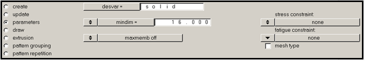
 to return to the Design History page, indicating that the
results correspond to optimization iterations.
to return to the Design History page, indicating that the
results correspond to optimization iterations.
 to open the Contour panel.
 to open the Iso Value panel.