Train Models
Train models using any physics, any mesh, and without design variable parametrization.
- Inclusion of a Dataset (number of samples and number of elements and time steps per sample)
- Model specifications (model size, hyperparameters, number of training epochs)
- Hardware (processor speed, RAM, access to GPU)
Training can also be done on an HPC. See Train Remotely on an HPC for more information.
-
From the PhysicsAI ribbon, select the Train
an ML Model tool.
Figure 2. 
The Train Model dialog opens. -
Define the training details and click Train.
-
Specify the hyperparameters of the training process, such as the number
of epochs or learning rate.
Note: You can hover over the hyperparameter names to read their description.
Hyperparameters will affect the quality of a trained model. The optimal set of hyperparameters will vary from problem to problem. Running experiments to the tune the hyperparameters to maximize model performance is an important last step in a complete physicsAI process.
Transfer learning involves using the knowledge from an existing physicsAI model while training a new model. It can be beneficial in cases where too few data points are available for training a new model from scratch. To enable transfer learning, the new phyicsAI model should have the exact same width, depth, and input features.
Figure 3. 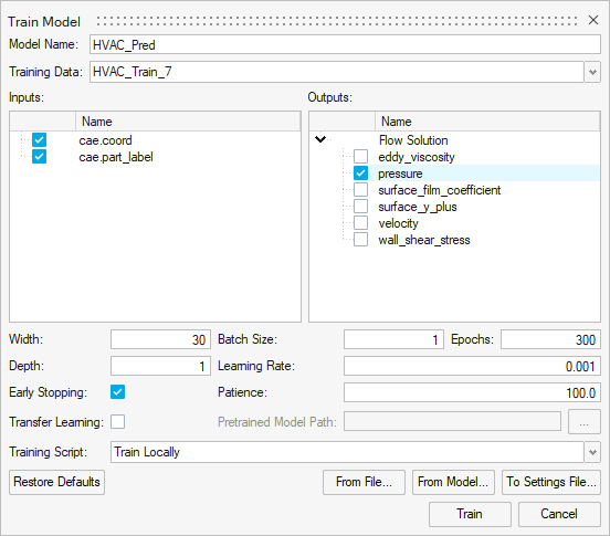
The Model Training dialog opens.
-
Specify the hyperparameters of the training process, such as the number
of epochs or learning rate.
-
Review the status in the Status column.
Tip: Once the status changes to Running, you can view the training logs by clicking Show Log.
Figure 4. 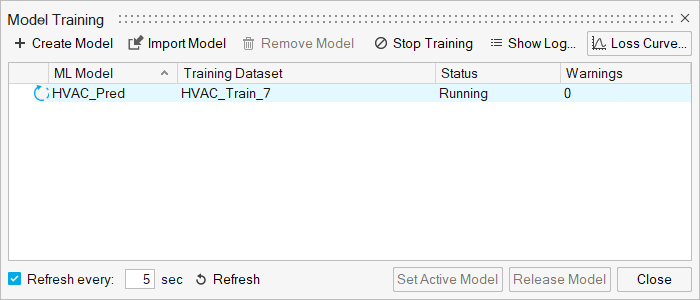
- Optional:
Click Loss Curve to view the training of a validation
loss curve.
The curves are useful to visualize the progress of the training process. In a well fit model, the training and validation losses become nearly identical. If validation never approaches the training loss, this is indicative of underfitting; increased training time can leave files d to improved model performance. A validation loss that approaches the training loss but diverges higher likely indicates overfitting; the point of low validation loss is the ideal model to avoid loss of generalization.Note: The validation curve only appears if there are at least 15 samples.
Figure 5. 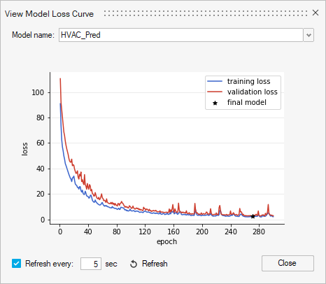
Train Remotely on an HPC
Train a PhysicsAI model on a remotely on a different machine than the one running the PhysicsAI GUI.
- Access to a remote machine with the Engineering Data Science (EDS) application installed
- PuTTY installed on your local machine
- A training script (details below)
- A mapped drive which can be accessed by both your local machine and the HPC. This is required so that your locally created datasets are visible to the HPC during training.
A common reason for remote training is to harness an HPC with a GPU, which can accelerate training significantly.
- Install the EDS application from the AltairOne Marketplace to your HPC.
-
Create an SSH connection.
- Launch PuTTY on your local machine and connect to the HPC via SSH.
- Save the connection, for example: my_physicsAI_hpc.
Important: If you are required to enter a password while logging in via PuTTY, you will need to setup RSA keys before continuing. Once you can login via PuTTY without entering a password, you may continue. -
Write a training script for your HPC using the following template.
This example uses the qsub command from PBS on Windows. For Windows, the script should have the .bat extension. If your local machine is running Linux, you will need to write a script with equivalent functionality on Linux with a .sh extension.
Below is a Linux example. This example script is setup under the assumption that you can already submit from your command terminal.@echo off SETLOCAL REM ------------------------------------------------------------------------------ REM Copyright (c) 2021 - 2021 Altair Engineering Inc. All Rights Reserved REM Contains trade secrets of Altair Engineering, Inc. Copyright notice REM does not imply publication. Decompilation or disassembly of this REM software is strictly prohibited. REM ------------------------------------------------------------------------------ REM ------------------------------------------------------------------------------ REM USER SETTINGS REM ------------------------------------------------------------------------------ REM HPC Setup set sess=<<HOST NAME>> set user=<<USER NAME>> REM PBS Requests set pbs_requests=-q a100 -N physicsAI_shape -j oe -l select=1:ncpus=8:mem=257940mb:ngpus=1 REM Windows -> Unix Mapping set win_map=\\<<SERVER IP>>\data\ds set unix_map=/data/ds REM PhysicsAI Installation Settings set install_loc=<<HW INSTALL LOCATION>>hwdesktop/hw/eds/bin/linux64/edspy.sh REM PBS Install Location set sub_cmd=/altair/pbsworks/pbs/exec/bin/qsub REM ------------------------------------------------------------------------------ REM SCRIPT START REM ------------------------------------------------------------------------------ REM Get whole input line set line=%* REM Map windows paths to unix set unixmap=%win_map%=%unix_map% set unixmap=%unixmap:\=/% set submit_line=%line:\=/% setlocal EnableExtensions EnableDelayedExpansion set submit_line=!submit_line:%unixmap%! echo %line% echo ---UNIXMAP--- IF ["%unixmap%"] == [""] GOTO :RUN setlocal EnableExtensions EnableDelayedExpansion :RUN echo ---PLINK SETTINGS--- echo user = %user% echo sess = %sess% echo ---PAI-SHAPE SETTINGS-- echo install_loc = %install_loc% echo submit_line = %submit_line% REM ----------------- REM Run QSUB REM ----------------- set qsub_command_string='%install_loc% %submit_line%' REM Write File for submission echo plink -load %sess% -l %user% -batch "echo %qsub_command_string% > pai_qsub.txt" plink -load %sess% -l %user% -batch "echo %qsub_command_string% > pai_qsub.txt" REM Submit file plink -load %sess% -l %user% -batch "%sub_cmd% %pbs_requests% pai_qsub.txt" echo plink -load %sess% -l %user% -batch "qsub %pbs_requests% pai_qsub.txt" ENDLOCAL#!/bin/tcsh # ------------------------------------------------------------------------------ # USER SETTINGS # ------------------------------------------------------------------------------ set pbs_requests="-q a100 -N physicsAI_shape -j oe -l select=1:ncpus=8:mem=250000mb:ngpus=1" echo ${pbs_requests} # Hyperworks Install Location set install_loc="/stage/hw/2024" echo ${install_loc} # PBS qsub install location set sub_cmd="/opt/pbs/bin/qsub" # ------------------------------------------------------------------------------ # SCRIPT START # ------------------------------------------------------------------------------ set submit_line="$*" echo submit_line = ${submit_line} set edspy=\$'{'install_loc'}'"/altair/hwdesktop/hw/eds/bin/linux64/edspy.sh" set qsub_command_string="export INSTALL_LOCATION=${install_loc};export install_loc=${install_loc}; ${edspy} ${submit_line}" echo qsub_command_string = ${qsub_command_string}; # Write the qsub sumbmission script. # If your home directory is not seen by the HPC, modify the location to be visible on the HPC or run command via ssh. echo "${qsub_command_string}" > ~/pai_qsub.txt; # Submit the qsub sumbmission script. # If you cannot directly submit to pbs, run this command via ssh. echo "qsub ${pbs_requests} pai_qsub.txt"; qsub ${pbs_requests} ~/pai_qsub.txt -
Register the training script.
-
From the PhysicsAI ribbon, select the
Train an ML Model tool.
Figure 6.
The Train Model dialog opens. -
Click
 and browse and
select your training script.
and browse and
select your training script.
Your preferences are saved and the physicsai_solver_prefs.json file in your user directory has been updated. -
From the PhysicsAI ribbon, select the
Train an ML Model tool.
-
Launch a remote training.
Your training script is invoked with the specified training dataset and model settings.
A training will begin running on your HPC.
Train Using a GPU
Training a PhysicsAI model on a GPU is significantly faster. To train a model on a GPU, locally or on an HPC, you must complete the following steps.
-
Install the NVIDIA CUDA toolkit and Deep Neutral Network library (CuDNN).
Once these tools are installed, the GPU will be used by default for both training and predicting. You can verify this in the Task Manager by enabling the cuda graph in the GPU Performance tab.
- To use the CPU again, set CUDA_VISIBLE_DEVICES=-1 as an environment variable.