In this tutorial you will learn how to setup an optimization problem using MotionView's Optimization Wizard for an impact absorber.
You will learn about the following:
Defining stiffness and damping of SpringDamper element as design variables
Defining responses of type MaxVal
Using the responses as objectives
Running the optimization and post-processing the results
Introduction
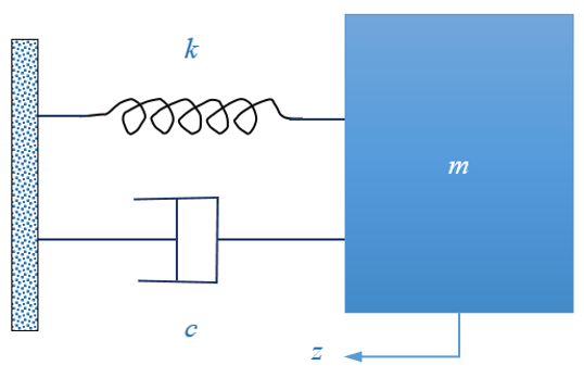
An impact absorber is modeled as a single degree of freedom system with a
mass m, a linear stiffness k and a linear damping coefficient c. The
velocity of the mass is 1 m/s; Mass m = 1 kg and a transient analysis end
time of 12 seconds is used.Figure 1. The objective of the optimization is to minimize the maximum
acceleration of the mass in the time interval 0 to 12s subject to the
condition that the maximum displacement is less than 1m. In order to achieve
this, stiffness k and damping ratio c are modeled as design variables.
MotionSolve's FD (Finite Differencing)
capability is used to calculate sensitivities.
Add Design Variables
In this step, you will add design variables for the optimization.
Before you begin, copy the file
mv_3021_initial_impact_absorber.mdl located in the
mbd_modeling\motionsolve\optimization\MV-3021 into your
<working directory>.
Open mv_3021_initial_impact_absorber.mdl in MotionView.
In the Project Browser, right-click on
Model and select Optimization
Wizard from the context menu.
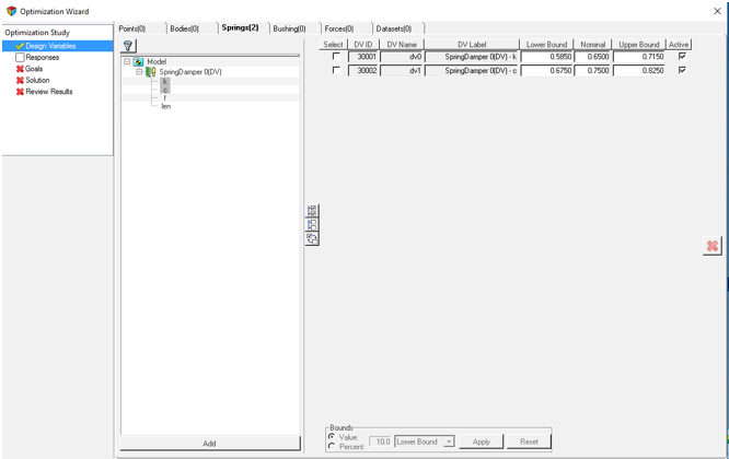
Under the Design Variables page, click on the
Springs tab.
Make the k and c of SpringDamper
0 design variables. Select k and c
datamembers from the Model Tree under the spring damper
and click Add.
Figure 2.
Modify the upper and lower bounds of the design variables according to Table 1.
Table 1.
DV
Lower Bounds
Upper Bounds
sd_0.k
0.2
1.0
sd_0.c
0.2
1.0
Add Response Variables
In this step you will add response variables for the optimization.
The objective of the optimization is to minimize the maximum acceleration while
keeping the displacement of mass to be less than 1.0. To achieve this, two responses are
created:
Maximum z direction acceleration of mass
Maximum z direction displacement of mass
The maximum z-direction acceleration response is used to define an objective; the
maximum z-direction displacement is used to define a constraint. Both responses are
created using ‘MaxVal’ response. This response can be used to capture the maximum value
of an expression throughout the simulation. The details of ‘MaxVal’ response can be
obtained from the ‘Multibody Optimization User’s Guide’ and the ‘MotionSolve User’s Guide’.
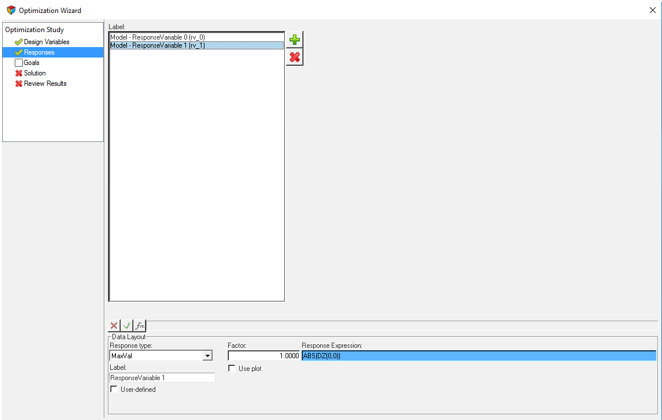
Click on the Responses page.
Click to add a response variable. Retain the default Label
and Variable name and click OK.
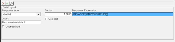
Once the response variable is created, under Response Type, choose
MaxVal.
In the Response Expression field, enter
`ABS(ACCZ({b_0.cm.id},{m_0.id}))` (the absolute value of
ACCZ of CM of Mass).
The Response Variable should look as shown in Figure 3:Figure 3.
Follow these steps again to create a second 'MaxVal' response. Use the Response
Expression `ABS(DZ({b_0.cm.id},{m_0.id}))`.
You have created all the necessary Response Variables. The completed
page will look as shown in Figure 4:Figure 4.
Add Objectives and Constraints
Now you will add objectives and constraints to the problem.
You can use the responses you created in the previous section as
objectives.
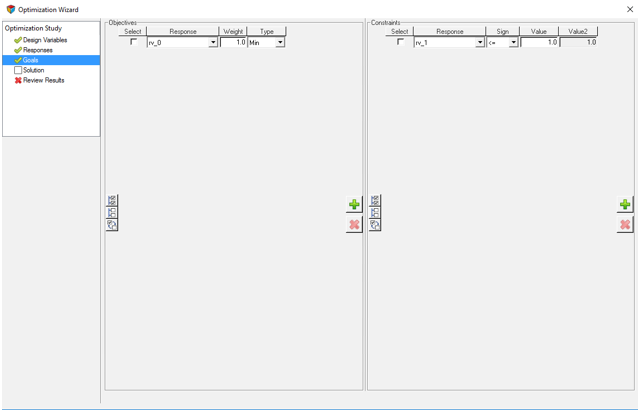
Navigate to the Goals page. Under Objectives, click
.
This will add an objective with the response rv_0.
Choose a Weight of 1.0 and retain the Type as
Min.
Under Constraints, click and modify the created response
rv_0 to be rv_1.
Retain the sign as '< =' and type 1.0 for value.
This will ensure that the value of rv_1 is less than 1.0. Now all
objectives and constraints are defined, and the model is ready to run. Figure 5.
Run the Optimization
In this step you will run the optimization.
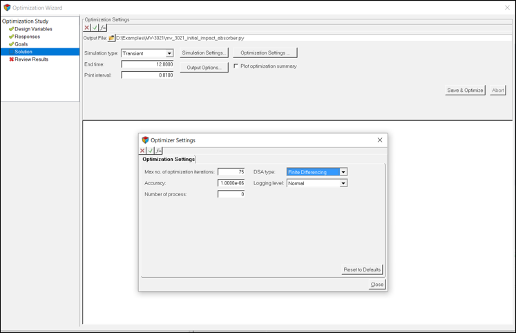
Navigate to the Solutions page to specify optimization
settings and run the analysis.
Click Optimization Settings.
Change the DSA type to FD.
Note: You also have the option to choose AUTO. When you choose AUTO, MotionSolve will detect the simulation type and
choose the best approach to compute sensitivity. The simulation type is
dynamic, so MotionSolve will choose FD.
Figure 6.
Click Save & Optimize to start the
optimization.
While the optimization is running, a plot of total weighted cost vs.
iteration number and constraint value is displayed in a separate
window.
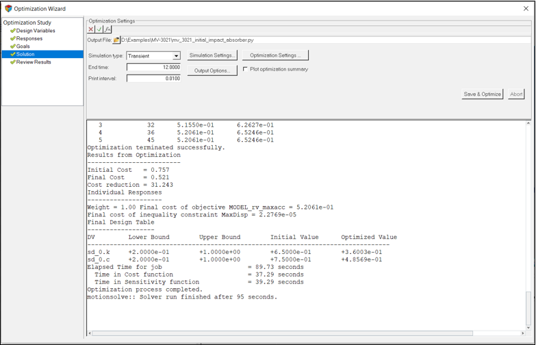
Once the optimization process is complete, the text window in
the Solution page displays the optimized design
variables values, final value of the responses and optimized cost
function.
Figure 7. The expected values of design variables are provided in Table 2:
Table 2.
RV/VD
Expected
From Optimizer
rv_0
0.5206
0.5206
sd_0.k
0.3606
0.36003
sd_0.c
0.4851
0.48569
Post-Process
In this step, you will post-process the optimization results of the impact
absorber.
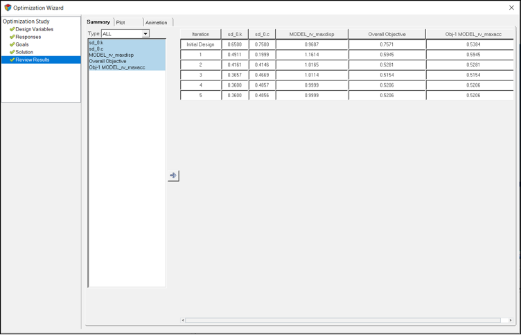
Navigate to the Review Results page.
The Summary tab is displayed with lists of values for design variables,
responses and objective being tabulated iteration-wise. For this tutorial, the
optimized design variables are from the last iteration 5.Figure 8.
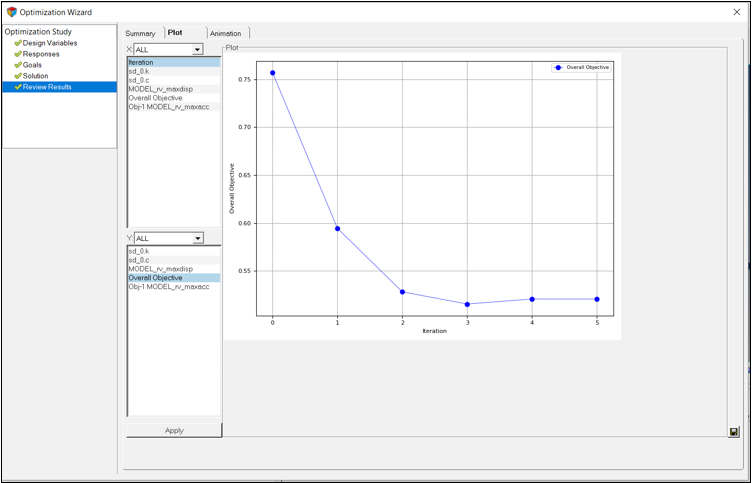
Click the Plot tab to visualize variation of design
variables, response variables and cost function using graphs.
Figure 9.
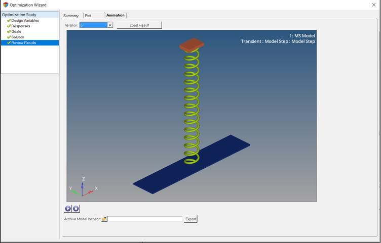
Click the Animation tab to animate the configuration
generated during any iteration.
Choose Iteration 5 and click on Load
Result to load the H3D file from that iteration.
You can click the / buttons to start and stop the animation.Figure 10. From this tab, you can also export an archive of the model in a state
corresponding to any iteration.
Click the Archive Model Location browser to specify a
file path.
Click the Export button.
This will create an archive folder which contains all files necessary to
open/run/optimize the model. The design variable values are set to the values in
the iteration number you choose.

 to add a response variable. Retain the default Label
and Variable name and click OK.
to add a response variable. Retain the default Label
and Variable name and click OK.
 /
/ buttons to start and stop the animation.