OS-T:2095 矩形プレートの周波数応答解析
本チュートリアルでは、OptiStructを用いた周波数応答最適化について解説します。
まず最初に、既存の平板の有限要素(FE)モデルを読み込み、モーダル法による周波数応答解析によってピーク振幅を求めます。続いて、同じプレートに対し過渡応答最適化を実行して新規設計案を得ます。
- 目標
- 体積の最小化
- 制約条件
- Max FRF Disp.< 600 mm
- 設計変数
- 設計空間内の各要素の密度
HyperMeshの起動とOptiStructユーザープロファイルの設定
-
HyperMeshを起動します。
User Profilesダイアログが現れます。
-
OptiStructを選択し、OKをクリックします。
これで、ユーザープロファイルが読み込まれます。ユーザープロファイルには、適切なテンプレート、マクロメニュー、インポートリーダーが含まれており、OptiStructモデルの生成に関連したもののみにHyperMeshの機能を絞っています。
モデルの読み込み
-
をクリックします。
Importタブがタブメニューに追加されます。
- File typeにOptiStructを選択します。
-
Filesアイコン
 を選択します。
Select OptiStruct Fileブラウザが開きます。
を選択します。
Select OptiStruct Fileブラウザが開きます。 - 自身の作業ディレクトリに保存したfrf_response_input.femファイルを選択します。
- Openをクリックします。
- Import、続いてCloseをクリックし、Importタブを閉じます。
荷重と境界条件の適用
SPCと単位荷重コレクターの作成
-
SPC荷重コレクターを作成します。
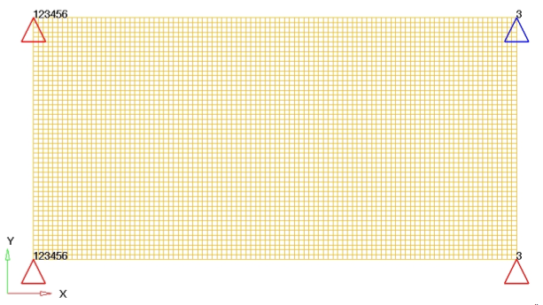
図 2. 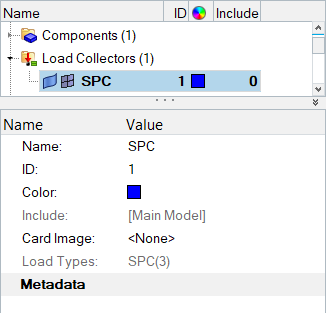
-
unit-load荷重コレクターを作成します。
拘束の作成
-
Model BrowserのCollectorsフォルダーでSPCを右クリックし、context menuからMake Currentを選択します。
図 3. 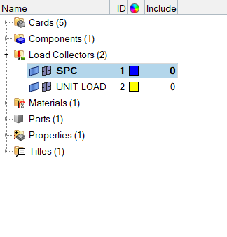
- Toolページからnumbersをクリックしてnumbersパネルを開きます。
- 拡張エンティティ選択メニューからを選択します。
- 次の数字を入力します:1、2、3、および4
- onをクリックします。
- returnをクリックします。
- Analysisページからパネルconstraintsをクリックします。
- パネル左側のラジオボタンを用いてcreateサブパネルが選択されていることを確認します。
-
Nodesをクリックし、IDで節点1と2を選択します。
-
IDが4の節点に制約条件を付与します。
- 節点セレクターを使って、IDが4の節点を選択します。
- dof3を除いた全ての自由度からチェックマークを外します。
- createをクリックします。
-
平板の1点への単位荷重の生成
- Model BrowserのCollectorsフォルダーでunit-loadを右クリックし、context menuからMake Currentを選択します。
- Constraintsパネルで節点コレクターを使って、IDが3の節点を選択します。
- dof3を除いた全ての自由度からチェックマークを外します。
- dof3=欄に20と入力します。
- load types=をクリックしDAREAを選択します。
- createをクリックします。
- returnをクリックし、メインメニューに進みます。
周波数範囲カーブの生成
-
Model Browserで右クリックしてを選択します。
Curve Editorが開きます。
- Curve editorウィンドウが表示されます。Newをクリックし、Name=にtabled1と入力してproceedをクリックします。
-
表に以下の値を入力してください:
- x(1)欄に0.0と入力します。
- y(1)欄に1.0と入力します。
- x(2)欄に1000.0と入力します。
- y(2)欄に1.0と入力します。
- 右上の X をクリックしてダイアログを終了します。
図 5. 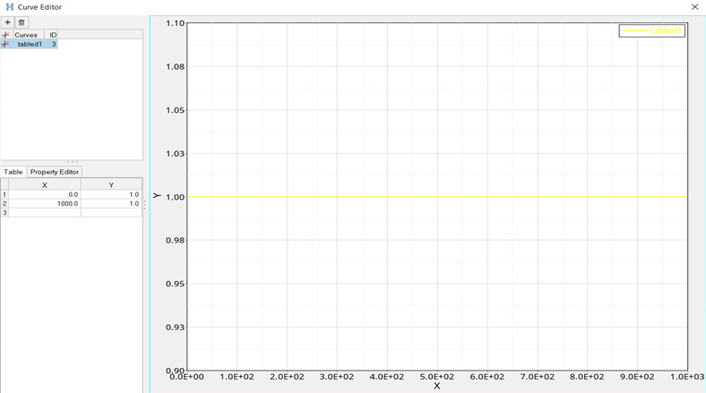
これで、周波数域0.0から1000.0まで、この範囲での一定値荷重が設定されました。
- Colorをクリックし、カラーパレットから色を選択します。
- Card ImageをTABLED1に設定します。
周波数依存動的荷重の作成
- Model Browser内で右クリックし、を選択します。
- Curve editorウィンドウが表示されます。Newをクリックし、Name=にrload2と入力してproceedをクリックします。
- Config typeにDynamic Load - Frequency dependentを選択します。
- Typeに、RLOAD2を選択します。
-
EXCITEIDを定義します。
- をクリックします。
- Select Loadcolダイアログでunit-loadを選択し、OKをクリックします。
-
TBを定義します。
- Curvesをクリックします。
- Select Curvesダイアログで、tabled1を選択し、OKをクリックします。
-
TYPEをLOADに設定します。
これは、入力をフォースに定義します。
応答の解に用いる周波数セットの生成
-
Model Browserで右クリックしcontext menuからを選択します。
デフォルトの荷重コレクターがEntity Editorに表示されます。
- Curve editorウィンドウが表示されます。Newをクリックし、Name=にfreq5と入力してproceedをクリックします。
- Colorをクリックし、カラーパレットから色を選択します。
- Card ImageをFREQiに設定します。
- FREQ5を選択します。
- NUMBER_OF_FREQ5=欄に1と入力します。
- FREQ5_MAX_NUMBER_OF_FR=欄に3と入力します。
-
Data: IDの横の
 をクリックします。
-
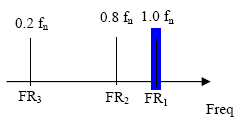
NUMBER OF FREQ =ダイアログで、周波数の値を定義します。
- F1欄に1.0と入力します。
- F2欄に1000と入力します。
- FR(0)欄に1.0と入力します。
- FR(1)欄に0.8と入力します。
- FR(2)欄に0.2と入力します。
- ダイアログを閉じるには、Closeをクリックします。
図 6. 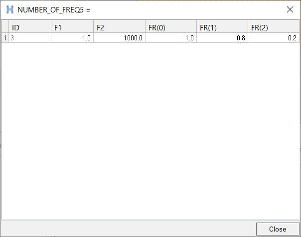
EIGRL荷重ステップ入力の作成
モーダル法として使用するEIGRL荷重ステップ入力を作成します。
- Model Browserで右クリックしてを選択します。
- Nameにeigrlと入力します。
- Config typeにReal Eigen Value Extraction を選択します。
- Typeに、EIGRLを選択します。
-
NDに17と入力します。
これで、Lanczos法を用いた最初の17の周波数の固有値抽出が指定されます。
荷重ステップの作成
- Analysisページからloadstepsをクリックします。
- Curve editorウィンドウが表示されます。Newをクリックし、Name=にsubcase1と入力してproceedをクリックします。
- typeをクリックし、Freq. resp (modal)を選択します。
-
SPCを定義します。
- SPCの前のボックスにチェックを入れます。
- 等号(=)をクリックして、荷重コレクターリストからspcを選択します。
-
METHOD(STRUCT)を定義します。
- METHOD (STRUCT)の前のボックスにチェックを入れます。
- 等号(=)をクリックして、荷重ステップ入力リストからeigrlを選択します。
-
DLOADを定義します。
- DLOADの前のボックスにチェックを入れます。
- 等号(=)をクリックして、荷重ステップ入力リストからrload2を選択します。
-
FREQを定義します。
- FREQの前のボックスにチェックを入れます。
- 等号(=)をクリックして、荷重コレクターリストからfreq5を選択します。
-
createをクリックします。
図 8. 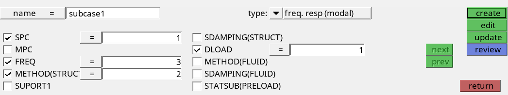
-
editをクリックし、RESVECを定義します。
- RESVECを選択します。
- TYPEをAPPLOADに設定します。
- OPTIONをYESに設定します。
spc荷重コレクター内の拘束条件とrload2荷重ステップ入力内の単位荷重をfreq5荷重コレクターで定義された周波数セットおよびeigrl荷重ステップ入力で定義されたモーダル法と共に参照するOptiStructサブケースが作成されました。
FRFシミュレーションの前にモーダル解析を行うことが推奨されます。ここでは、Frequency Response Analysisのセットアップに焦点を当てるため、この手順は省略します。
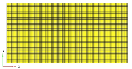
出力結果のための節点セットの生成
-
Model Browserで右クリックしcontext menuからを選択します。
デフォルトのセットがEntity Editorに表示されます。
- NemeにSETAと入力します。
- Card ImageをSET_GRIDに設定します。
- Set Typeをnon-orderedにセットします。
- Entity IDsに、.をクリックします。
-
節点セレクターを使って、IDが3の節点を選択します。
これで、集中荷重がかかる節点が選択されます。
- パネル領域で、proceedをクリックします。
- returnをクリックし、ダイアログを抜けます。
周波数応答解析用の出力と減衰のセットの作成
-
Analysisページからパネルcontrol cardsをクリックします。
Card Imageダイアログが開きます。
-
GLOBAL_OUTPUT_REQUESTを定義します。
-
SID(1)をダブルクリックし、SETAを選択します。
値1がSID入力ボックスの下に現れます。これは、set 1内の節点に限った出力を設定しています。
図 9. 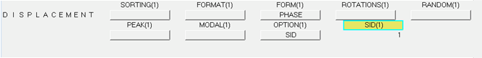
-
SID(1)をダブルクリックし、SETAを選択します。
-
FORMATを定義します。
- FORMATをクリックします。
- number_of_formats=欄に2と入力します。
- FORMAT_V1の下で、2回目のFORMATをクリックし、OPTIを選択します。
- returnをクリックします。
-
PARAMを定義します。
-
OUTPUTを定義します。
- OUTPUTをクリックします。
- KEYWORDをHGFREQに設定します。
- FREQをLASTに設定します。
- number_of_outputs=を1に設定します。
- returnをクリックします。
- returnをクリックし、メインメニューに戻ります。
データベースの保存
- menu barでをクリックします。
- Save Asダイアログでファイル名欄にfrf_response_input.hmと入力し、自身の作業ディレクトリに保存します。
ジョブのサブミット
-
AnalysisページからOptiStructパネルをクリックします。
図 10. OptiStructパネルへのアクセス 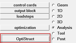
- save asをクリックします。
-
Save Asダイアログで、OptiStructモデルファイルを書き出す場所を指定し、ファイル名としてfrf_response_analysisと入力します。
OptiStruct入力ファイルには、拡張子 .femが推奨されます。
-
Saveをクリックします。
入力ファイル欄には、Save Asダイアログで指定されたファイル名と場所が表示されます。
- export optionsのトグルをallにセットします。
- run optionsのトグルをanalysisにセットします。
- memory optionsのトグルはmemory defaultにセットします。
- options欄を空にします。
- OptiStructをクリックし、OptiStructジョブを開始します。
結果の表示
- OptiStructパネル内でHyperViewをクリックし、解析からの結果を次のページに読み込みます。
- menu barでをクリックします。
-
Open Session Fileダイアログで、ジョブが実行されたディレクトリに進み、frf_response_analysis_freq.mvwファイルを開きます。
- オプション: OptiStructパネルから起動した場合、Yesをクリックして、現在のセッションを破棄します。
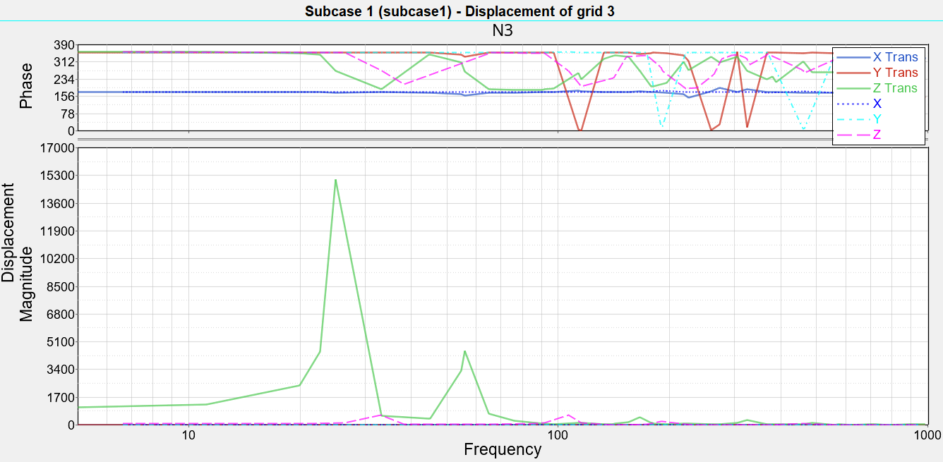
2つのグラフが表示されます。グラフのタイトルは、Subcase 1(subcase1)-Displacements of grid 3です。上のグラフはPhase Angle verses Frequency(位相角vs周波数)、下のグラフは、変位振幅vs周波数を示しています。図 11. 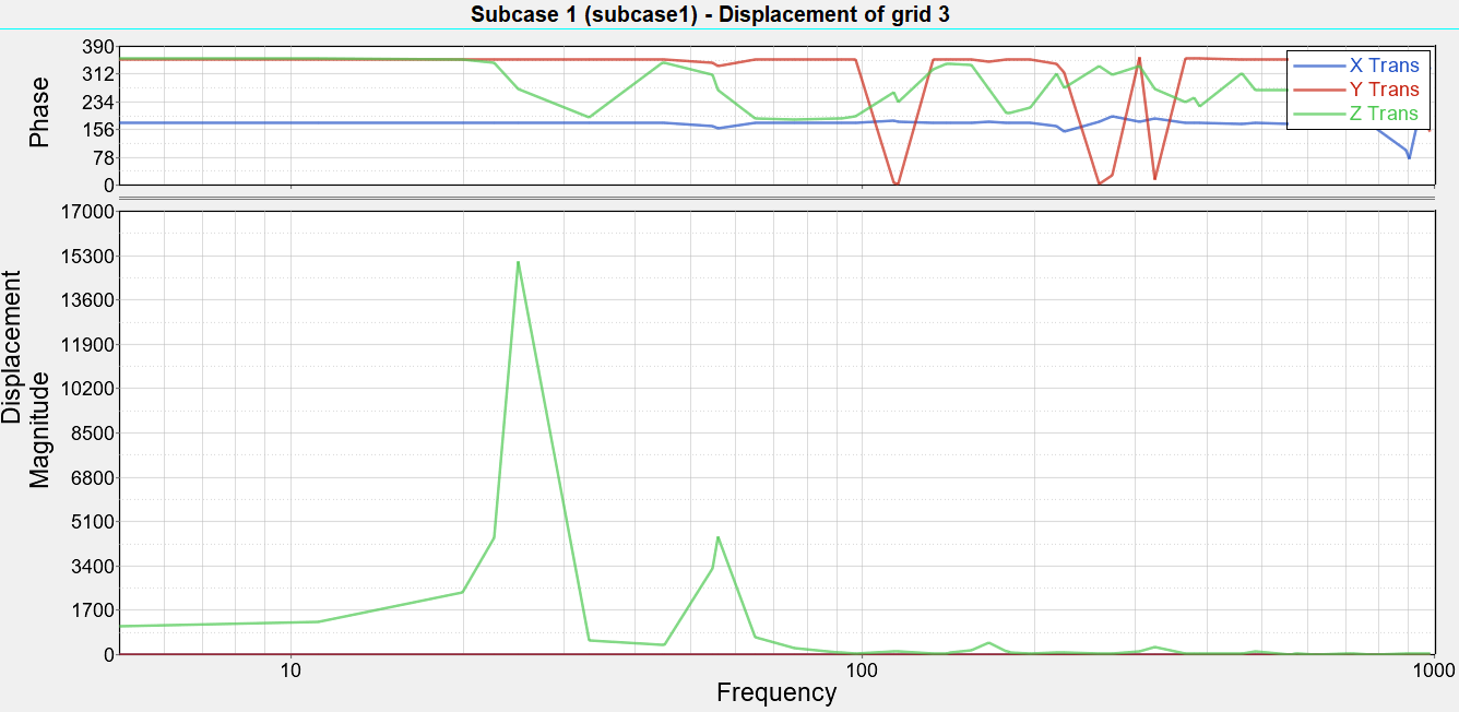
-
Curvesツールバーで
 をクリックし、Define Curvesパネルを開きます。
-
X TransおよびY Transカーブを消去します。
励振はZ方向にかかり、主効果はこの方向で検知されます。
-
Resultsツールバーで
 をクリックし、Curve Attributes パネルを開きます。
-
ラインの属性を連続
 に変更します。
-
Symbol Attributesタブで、正方形のシンボルを選択します。
図 12. 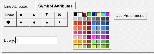
-
Annotationsツールバーで
 をクリックし、Axesパネルを開きます。
-
AxisをVerticalに変更します。
図 13. 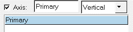
- Scale and Tics (Magnitude)タブをクリックしてLogarithmicを選択します。
- Min欄に5と入力します。
- Max欄に200000と入力します。
- Scale and Tics (Phase)タブをクリックし、Tics per axisを7に変更します。
-
AxisをHorizontalに設定します。
図 14. 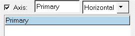
- Min欄に5と入力します。
-
Max欄に1000と入力します。
図 15. 周波数応答関数 FRF (Node 3, Z-Displacement) 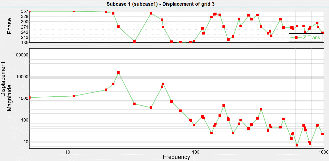
-
Curvesツールバーで
 をクリックし、Coordinate Infoパネルを開きます。
-
Find pointの下でMagnitudeを選択します。
図 16. 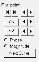
-
maximumボタンをクリックし、表内でY-magnitudeの最大値が15055であることを確認します。ベースラインモデルのピーク変位。
図 17. 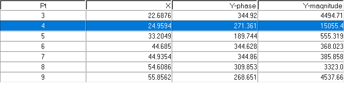
-
クライアントセレクターを
 に変更することで、HyperMeshに戻ります。
モデルのオープン
- をクリックします。
- 自身の作業ディレクトリに保存したfrf_response_input.hmファイルを選択します。
-
Openをクリックします。
frf_response_input.hmデータベースが現在のHyperMeshセッションに読み込まれます。
データベースの保存
- menu barでをクリックします。
- Save Asダイアログでファイル名欄にfrf_response_optimization.hmと入力し、自身の作業ディレクトリに保存します。
最適化のセットアップ
Create Topology Design Variables
- From the Analysis page, click optimization.
- Click topology.
- Select the create subpanel.
- In the desvar= field, enter plate.
- Set type: to PSHELL.
- Using the props selector, select Design.
- For base thickness, enter 0.15.
-
Click create.
A topology design space definition, shield, has been created. All elements referring to the design property collector (elements organized into the "design" component collector) are now included in the topology design space. The thickness of these shells can vary between 0.15 (base thickness) and the maximum thickness defined by the T (thickness) field on the PSHELL card.
The object of this exercise is to determine where to locate ribs in the designable region. Therefore, a non-zero base thickness is defined, which is the original thickness of the shells. The maximum thickness, which is defined by the T field on the PSHELL card, should be the allowable depth of the rib.
Currently, the T field on the PSHELL card is still set to 0.15 (the original shell thickness). You will change this to a higher value to create a design space where the material can be removed.
-
Update the design variable's parameters.
- Select the parameters subpanel.
- Toggle minmemb off to mindim=, then enter 2.0.
- Toggle maxmemb off to maxdim=, then enter 6.0.
- Click update.
- Click return.
-
Edit the thickness of the design property.
- In the Model Browser, Properties folder, click design.
- In the Entity Editor, T field, enter 1.000.
Create Optimization Responses
- From the Analysis page, click optimization.
- Click Responses.
-
Create the volume response, which defines the volume fraction of the design
space.
- In the responses= field, enter volume.
- Below response type, select volume.
- Set regional selection to total and no regionid.
- Click create.
-
Create the frequency response displacement (constraint), which defines the
maximum magnitude on dof3.
- In the responses= field, enter frfdisp.
- Set the response type to frf displacement.
- Switch the component from real to magnitude.
- Set the function to all freq.
- Using the nodes selector, select the node with ID 3.
- Select dof3.
- Click create.
- Click return to go back to the Optimization panel.
Create Design Constraints
- Click the dconstraints panel.
- In the constraint= field, enter constr.
- Click response = and select frfdisp.
- Check the box next to upper bound, then enter 600.
- Using the loadsteps selector, select subcase1.
- Click create.
- Click return to go back to the Optimization panel.
Define the Objective Function
- Click the objective panel.
- Verify that min is selected.
- Click response= and select volume.
- Click create.
- Click return twice to exit the Optimization panel.
Run the Optimization
- From the Analysis page, click OptiStruct.
- Click save as.
-
In the Save As dialog, specify location to write the
OptiStruct model file and enter
frf_response_optimization for filename.
For OptiStruct input decks, .fem is the recommended extension.
-
Click Save.
The input file field displays the filename and location specified in the Save As dialog.
- Set the export options toggle to all.
- Set the run options toggle to optimization.
- Set the memory options toggle to memory default.
-
Click OptiStruct to run the optimization.
The following message appears in the window at the completion of the job:
OPTIMIZATION HAS CONVERGED.
FEASIBLE DESIGN (ALL CONSTRAINTS SATISFIED).
OptiStruct also reports error messages if any exist. The file frf_response_optimization.out can be opened in a text editor to find details regarding any errors. This file is written to the same directory as the .fem file. - Click Close.
- frf_response_optimization.hgdata
- HyperGraph file containing data for the objective function, percent constraint violations, and constraint for each iteration.
- frf_response_optimization.HM.comp.tcl
- HyperMesh command file used to organize elements into components based on their density result values. This file is only used with OptiStruct topology optimization runs.
- frf_response_optimization.HM.ent.tcl
- HyperMesh command file used to organize elements into entity sets based on their density result values. This file is only used with OptiStruct topology optimization runs.
- frf_response_optimization.html
- HTML report of the optimization, giving a summary of the problem formulation and the results from the final iteration.
- frf_response_optimization.oss
- OSSmooth file with a default density threshold of 0.3. You may edit the parameters in the file to obtain the desired results.
- frf_response_optimization.out
- OptiStruct output file containing specific information on the file setup, the setup of the optimization problem, estimates for the amount of RAM and disk space required for the run, information for all optimization iterations, and compute time information. Review this file for warnings and errors that are flagged from processing the frf_response_optimization.fem file.
- frf_response_optimization.sh
- Shape file for the final iteration. It contains the material density, void size parameters and void orientation angle for each element in the analysis. This file may be used to restart a run.
- frf_response_optimization.stat
- Contains information about the CPU time used for the complete run and also the break-up of the CPU time for reading the input deck, assembly, analysis, convergence, and so on.
- frf_response_optimization_des.h3d
- HyperView binary results file that contain optimization results.
- frf_response_optimization_s#.h3d
- HyperView binary results file that contains from linear static analysis, and so on.
- frf_response_optimization.his_data
- The OptiStruct history file containing iteration number, objective function values and percent of constraint violation for each iteration.
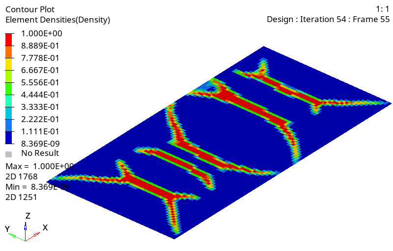
結果の表示
すべての反復計算における要素密度と要素板厚の結果がOptiStructから出力されます。
密度結果の静的プロットの表示
- OptiStructパネルから、HyperViewをクリックします。
-
frf_response_optimization.mvwセッションファイルを開きます。
- menu barでをクリックします。
- Open Session Fileダイアログで作業ディレクトリに移動し、frf_response_optimization.mvwセッションファイルを開きます。
-
Resultsツールバーで
 をクリックし、Contour panelを開きます。
-
Results Browserから、最終荷重ケースシミュレーションを選択します。
図 18. 
- Contour panelで、averaging methodをsimpleに設定します。
- applyをクリックします。
最適化実行結果のピーク変位の比較
-
FRF_response_analysis_freq.mvwセッションファイルを開きます。
- menu barでをクリックします。
- Open Session Fileダイアログで作業ディレクトリに移動し、FRF_response_analysis_freq.mvwセッションファイルを開きます。
-
Curvesツールバーで
 をクリックしてBuild Plotsパネルを開きます。これは、既存の解析情報に重ねて曲線を追加するために使用します。
-
Data file欄に、最終反復解析を含んだfrf_response_optimization_s2.h3d最適化ファイルを読み込みます。
図 20. 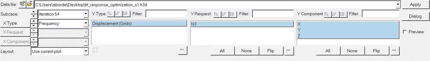
- Subcaseを最終反復計算に設定します。
- X TypeをFrequencyにセットします。
- Y Typeには、Displacement (Grids)を選択します。
- Y RequestにN3を選択します。
- Y ComponentにX、Y、Zを選択します。
- Applyをクリックし、新規情報を元のプロットに重ね書きします。