OS-T: 1070 Analysis of an Axi-symmetric Structure
In this tutorial the method of modeling an axi-symmetry problem in OptiStruct is covered.
Launch HyperMesh and Set the OptiStruct User Profile
-
Launch HyperMesh.
The User Profile dialog opens.
-
Select OptiStruct and click
OK.
This loads the user profile. It includes the appropriate template, macro menu, and import reader, paring down the functionality of HyperMesh to what is relevant for generating models for OptiStruct.
Open the Model
- Click .
- Select the axi-symmetry_full_geometry.hm file you saved to your working directory.
-
Click Open.
The axi-symmetry_full_geometry.hm database is loaded into the current HyperMesh session, replacing any existing data.
Exercise 1: Analysis with the Full Model
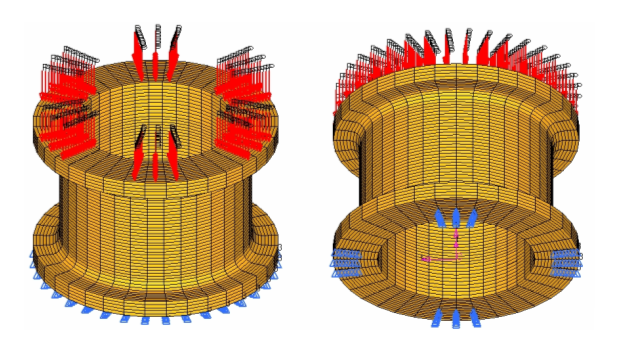
You will find that the structural model has already been set up with the necessary elements, boundary conditions, property, and material data so that it is ready to solve. Pressure load is applied on the top face of the geometry and constraints are defined at the bottom face. Note that the model is symmetrical about the z-axis and that loads and boundary conditions are symmetrical about the same axis as well. These represent the conditions necessary for modeling axi-symmetry problems. First, obtain the result for the full model and then you model a small part of the model with boundary conditions suitable to enforce the axi-symmetric behavior. Finally, you compare the results of the axi-symmetric model with the full model results.
Submit the Job
-
From the Analysis page, click the OptiStruct
panel.
Figure 2. Accessing the OptiStruct Panel 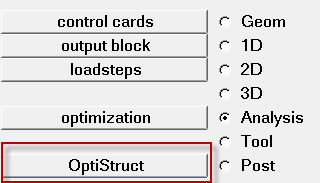
- Click save as.
-
In the Save As dialog, specify location to write the
OptiStruct model file and enter
axi-symmetry_full_geometry for filename.
For OptiStruct input decks, .fem is the recommended extension.
-
Click Save.
The input file field displays the filename and location specified in the Save As dialog.
- Set the export options toggle to all.
- Set the run options toggle to analysis.
- Set the memory options toggle to memory default.
- Click OptiStruct to launch the OptiStruct job.
View the Results
-
From the OptiStruct panel, click HyperView.
HyperView is launched and the results are loaded. A message window appears to inform of the successful model and result files loading into HyperView.
- Click Close to close the message window, if one appears.
View the Displacements of the Structure
- Set the Animation mode to Linear.
-
On the Results toolbar, click
 to open the
Contour panel.
to open the
Contour panel.
- Select the first pull-down menu below Result Type and select Displacement [v].
-
Select the second pull-down menu below Result Type and select
Mag.
Figure 3. 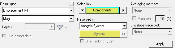
-
Click Apply to display the displacement contour.
Tip: To view the displacement variation across the thickness, one half of the structure can be masked.
- Expand the Components folder in the Results Browser.
- Click the elements icon in front of the component bottom_half to mask the component from display.
Figure 4. 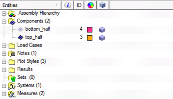
-
Click XZ Left Plane View
 to display the Left
view.
The following figure shows the displacements through the thickness.
to display the Left
view.
The following figure shows the displacements through the thickness.Figure 5. 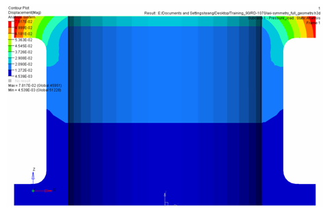
Exercise 2: Analysis with a Small Portion of the Full Model with Axi-symmetry Boundary Conditions
Set up the New Analysis
Return to HyperMesh to delete the all the elements, except for a small portion and to set up the axi-symmetry boundary conditions.
Set up the Axi-symmetry Model
-
Click
 to
enter the Delete panel, or click
F2.
to
enter the Delete panel, or click
F2.
- Make sure the entity selection switch is set to elems.
- Click the yellow button elems to open the extended entity selection window and select by sets.
-
Click in the check box in front of SetA.
A check mark appears before SetA to indicate that it is selected.
-
Click select.
The selected elements are highlighted.
- Click delete entity to delete the selected elements.
-
Click return to exit the Delete panel.
Use the retained portion to model the axi-symmetric model with suitable boundary conditions.
Apply the Additional Boundary Conditions
- From the Analysis page, enter the Systems panel.
- Select the assign radio button.
- Make sure the entity selection switch in front of set: is set to nodes.
- Click the yellow button nodes to open the extended entity selection window and select all.
- Click the yellow button system to activate it and select the red colored system from the modeling window.
-
Click set displacement.
The message on the footer bar The analysis system has been assigned appears.
- Click return.
Create Constraints
- Expand the Load Collectors folder in the Model Browser.
- Right-click on SPCs and click Make Current to make SPCs the current component, if not already done.
- Click to open the Constraints panel.
- Make sure the entity selection switch is set to nodes.
- Click the yellow button nodes to open the extended entity selection window and select all.
-
Constrain dof2.
- DOFs with a check will be constrained while DOFs without a check will be free.
- DOFs 1, 2, and 3 are x, y, and z translation degrees of freedom.
- DOFs 4, 5, and 6 are x, y, and z rotational degrees of freedom.
-
Click create.
This applies these constraints to the selected nodes.
- Click return to go back to the main menu.
- From the Analysis page, enter the OptiStruct panel.
-
Solve the job with file name as axi-symmetry_model.fem by
following the same steps as explained in the earlier section.
If the job is successful, new results files can be seen in the directory where the OptiStruct model file was written. The axi-symmetry_model.out file is a good place to look for error messages that will help to debug the input deck if any errors are present.
Submit the Job
-
From the Analysis page, click the OptiStruct
panel.
Figure 7. Accessing the OptiStruct Panel
- Click save as.
-
In the Save As dialog, specify location to write the
OptiStruct model file and enter
axi-symmetry_model for filename.
For OptiStruct input decks, .fem is the recommended extension.
-
Click Save.
The input file field displays the filename and location specified in the Save As dialog.
- Set the export options toggle to all.
- Set the run options toggle to analysis.
- Set the memory options toggle to memory default.
- Click OptiStruct to launch the OptiStruct job.
View the Results
- Click HyperView to view the results.
-
Click the Page Layout icon
 .
.
-
Select the two window layout
 .
.
- Activate the new window by clicking in the modeling window of the new window.
-
Click
 to open the Load Model and
Results panel.
to open the Load Model and
Results panel.
-
Click the Load model icon
 on the toolbar and load the
axi-symmetry_model.h3d.
This loads the complete path of the selected .h3d file in the field. Also, note that the same file path is loaded next to the field Load results.
on the toolbar and load the
axi-symmetry_model.h3d.
This loads the complete path of the selected .h3d file in the field. Also, note that the same file path is loaded next to the field Load results. - Click Apply.
-
Click XZ Left Plane View
to display the Left
view.
-
Click the Contour icon
 on the toolbar and contour the displacements.
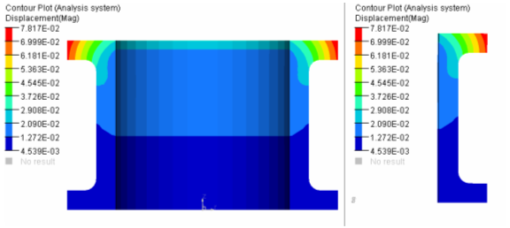
- Compare the displacement results of the axi-symmetry model with the result from the full model. The results should match, as shown in the below picture. Similarly, stress and other results will also match.
Figure 8. Comparison of Displacement Results