Create temperature constraints by applying a load that represents temperatures to
nodes, components surfaces, or sets.
Temperatures are load config 5 and are displayed as a vertical line with the letter T
at the top.
注: In the Radioss, Abaqus, and LS-DYNA profiles,
load entities are created immediately upon entering the tool. Use the エンティティエディター to modify any properties. In all other solver
profiles, load entities aren't created until you make your selections then click
Create.
From the Analyze ribbon, click the Temperatures
tool.
図 1.
Select the keyword to create from the Load Type menu.
The available types depend on the current solver interface.
Select entities to which temperatures will be applied.
In any case, the forces are applied to nodes; this selection simply determines
how those nodes are selected. For example, components select all of the nodes
contained within the chosen component.
Specify the magnitude and direction of the temperature.
Constant Value
The value of the load magnitude.
Curve
When working with loads that are time-dependent, specify the time
history of the load using a vector entity. When using this option,
you may choose to apply the load normal to the elements, or use the
plane and vector tool to specify a direction. Use the curve selector
to select the curve representing the load time history. This curve
must already exist in the model. The optional scale factor field
allows you to scale the X vector of the curve. Curves can be viewed
and modified from within the XY Plots module.
Equation
Specify the loading equation. Use the plane and vector tool to
specify a direction, then select the coordinate system to which the
vector corresponds.
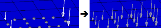
Field Loads
Interpolate and extrapolate loads from existing loads. You can then
select the desired elements to which you wish to add loads, and any
existing loads on which you wish to base additional forces.
When you create, HyperMesh uses a
Green's function with the given boundary loads in order to create
the loads on all of the selected nodes. For smoothness, the gradient
at the boundary points is enforced to be zero; this ensures that the
extrapolated loads remain lower than the input loads. For this
reason it is recommended to use representative boundary values as
input to be able to capture the peaks reasonably.
注: This version differs from linear
interpolation both in the way that the load magnitudes are
determined, and also in the fact that it can be applied to nodes
outside the boundaries of the chosen existing loads.
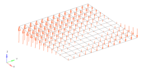
Linear Interpolation
Interpolate loads from a saved file or existing loads.
注: Only available for shell
elements.
Each row of the input file contains the x,y,z coordinates of the
load followed by its three components. The data can be separated by
a space or tab.
You can then select the desired nodes to which you wish to add
loads, and pick 3 or more existing loads that enclose those nodes.
When you interpolate, a linear function is used to create additional
loads on the selected nodes, with magnitudes based on the magnitudes
of the loads that you had selected.図 2.
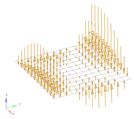
In the search radius field, specify the
search distance to find the loads which are within that distance
from a centroid or node on which a load is being interpolated. The
nearest 3 loads located within that distance are used to create the
load at the centroid or node by linear interpolation. Linear
interpolation uses a triangulation method, so if it finds fewer than
3 loads within that distance no interpolation takes place. While
reading the initial loads from a file, if linear interpolation is
not possible because the search radius is too small, the original
loads are simply applied to the nearest centroid or node.
Select fill gap to create a load at every
selected element centroid or node irrespective of the size of the
search radius.